Comparing Systems, Continued

Normal Means Selection

In this lesson, we will look at the classic problem of choosing the normal distribution having the largest mean. Furthermore, we'll guarantee a certain probability of correct selection.

Find the Normal Distribution with the Largest Mean

Let's start with some underlying assumptions. We will assume that we can take independent observations, $Y_{i1}, Y_{i2},..., Y_{in}, (1 \leq i \leq k)$, from $k \geq 2$ normal populations $\prod_1,...,\prod_k$. Here, $\prod_i$ refers to a normal distribution with unknown mean $\mu_i$ and known or unknown variance $\sigma_i^2$.

Let's denote the vector of means as $\boldsymbol \mu = (\mu_1,...,\mu_k)$ and the vector of variances as $\boldsymbol \sigma^2 = (\sigma^2_1,...,\sigma^2_k)$. Furthermore, let's denote the ordered (but unknown) $\mu_i$'s as $\mu_{[1]} \leq \cdots \leq \mu_{[k]}$.

We will refer to the "best" system as that which has the largest mean, $\mu_{[k]}$. Our goal is to select the population - strategy, treatment, alternative, etc. - associated with mean $\mu_{[k]}$. We make a correct selection (CS) if we achieve our goal.

Indifference-Zone Probability Requirement

For specified constants, $P^*$ and $\delta^*$, where $\delta^* > 0$ and $1/k < P^* < 1$ we require:

We want the probability of correct selection to be at least $P^*$, which we specify according to our sensitivity. Moreover, $P^*$ is in the range $(1/k, 1)$. The lower bound is $1/k$, not zero, because $1/k$ is the probability of correct selection given a random guess. Of course, $P$ cannot equal one unless we take an infinite number of samples.

On the other hand, $\delta^*$ merely has to be greater than zero, because its a bound on $\mu_{[k]} - \mu_{[k-1]}$, and $\mu_{[k]} > \mu_{[k-1]}$. Remember, we also specify $\delta^*$.

We can think about $\delta^*$ as the smallest difference worth detecting. When we specify a small $\delta^*$, we are saying that we want to catch very small differences between $\mu_{[k]}$ and $\mu_{[k-1]}$. As we increase $\delta^*$, we increase the difference between $\mu_{[k]}$ and $\mu_{[k-1]}$ that we are willing to tolerate.

As long as the difference between the two values is less than $\delta^*$, we don't care which we pick. Of course, if the difference between $\mu_{[k]}$ and $\mu_{[k-1]}$ is bigger than $\delta^*$, we want to make sure we select the right population.

Obviously, the probability of correct selection depends on the differences $\mu_i - \mu_j$, the sample size, $n$, and $\boldsymbol \sigma^2$.

Parameter configurations $\boldsymbol \mu$ satisfying the constraint $\mu_{[k]} - \mu_{[k-1]} \geq \delta^*$ are in the preference zone for correct selection. For example, if $\mu_{[k]} = 5$, $\mu_{[k-1]} = 3$, and $\delta^* = 1$, then the $\boldsymbol \mu$ containing this $\mu_{[k]}$ and $\mu_{[k-1]}$ would be in the preference zone.

If $\boldsymbol \mu$ falls in the preference zone, we want to ensure that we make the correct selection.

Parameter configurations $\boldsymbol \mu$ not satisfying the constraint $\mu_{[k]} - \mu_{[k-1]} \geq \delta^*$ are in the indifference zone. For example, if $\mu_{[k]} = 5$, $\mu_{[k-1]} = 3$, and $\delta^* = 3$, then the $\boldsymbol \mu$ containing this $\mu_{[k]}$ and $\mu_{[k-1]}$ would be in the indifference zone.

If $\boldsymbol \mu$ falls in the indifference zone, it doesn't matter too much if we choose $\mu_{[k-1]}$ over $\mu_{[k]}$, because the two values are within the threshold we've set.

Any procedure that guarantees equation $(1)$ above is said to be employing the indifference zone approach.

So Many Procedures

There are hundreds of different procedures we can use that implement this approach. Of note are the following:

• Bechhofer's Single-Stage procedure
• Rinott's Two-Stage procedure
• Kim and Nelson's Sequential procedure

We'll look at the basics of the single-stage procedure in the next lesson. As a word of caution, we wouldn't use this procedure in the wild. It relies on common, known variances among the competing populations, and we rarely know variances when running experiments.

Single-Stage Normal Means Procedure

In this lesson, we'll look at a specific, simple single-state procedure. The purpose of this light introduction is to give a taste of the kinds of procedures available for these types of general selection problems. As we said previously, this procedure assumes that all of the competing normal distributions have common, known variances, which is almost always an unrealistic assumption. Better procedures are out there.

Single-Stage Procedure

The single-stage procedure, $\mathcal{N}_\text{B}$, from Bechhofer, takes all necessary observations and makes a selection decision at once. It assumes that the populations have common, known variance, which is a fairly restrictive assumption.

For $k$ competing populations, with specified $P^*$ and $\delta^* / \sigma$, we determine a sample size $n$, usually from a table, such that our probability requirement is satisfied. Remember that $P^*$ and $\delta^*$ are the previously discussed parameters, and $\sigma$ is the known standard deviation.

Once we have $n$, we will take a random sample of $n$ observations $Y_{ij}, \enspace (1 \leq j \leq n)$ in a single stage from $\prod_i, \enspace (1 \leq i \leq k)$.

We then calculate the $k$ sample means:

We will select the population that yields the largest sample mean, $\bar Y_{[k]} = \max\{\bar Y_1,..., \bar Y_k\}$ as the one associated with $\mu_{[k]}$.

The procedure is very intuitive. All that remains is to figure out $n$. We can use a table or a multivariate normal quantile, or we can compute $n$ via a separate simulation if all else fails.

Let's take a look at the table:

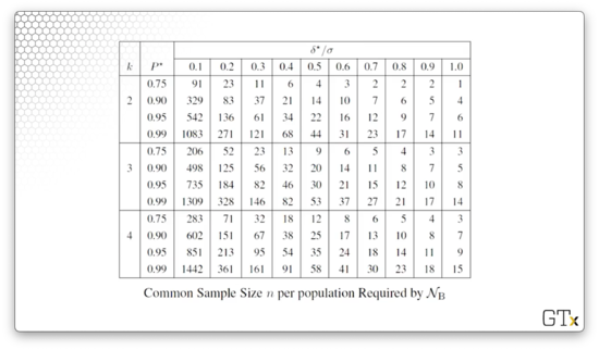
We can see the various parameters along the left and top axes, and the required value for $n$ in the corresponding cell. For instance, if we have $k=3$ competitors, and we want the probability of correct selection to be $P^* = 0.9$, and we want $\delta^* / \sigma = 0.5$, then we'll take $n=20$ observations.

If we don't want to use the table, we can directly calculate $n$ using a multivariate normal quantile:

Let's remember our probability requirement:

The value of $n$ satisfies the above requirement for any vector of unknown means, $\boldsymbol \mu$, having the following configuration:

This configuration is known as the slippage, or least-favorable, configuration. All of the inferior means are the same, and the best mean is $\delta^*$ better than the rest. This configuration is least-favorable because, for fixed $n$, it minimizes $P(\text{CS})$ among all $\boldsymbol \mu$ in the preference zone.

Proof

Let's look at a proof of how we calculate $n$. Let's start by defining $P^*$ as the probability of correct selection given that we are in the least-favorable configuration:

The correct selection is that population that has the true best mean. We can only make the correct selection if the sample mean corresponding to the true best mean is bigger than all the other sample means. Assuming the true best population is the $k$th one:

If we select population $k$, we better make sure that its sample mean is larger than the sample means from all other competing populations.

Let's standardize the right-hand side of the inequality by subtracting its true mean, $\mu_k$, whatever that may be, and dividing by its variance, $\sigma^2 / n$. Of course, we have to apply the same transformation to the left-hand side:

We know that the right-hand side of the inequality is a standard normal random variable. Let's call that $x$ now. We can condition it out by integrating over all $x$. Notice that we have to include the standard normal pdf, $\phi(x)$, in this integration:

Now, let's standardize the right-hand side of the inequality. We can't just subtract by $\mu_i$ since we are already subtracting by $\mu_k$, so we have to add an adjustment factor on the right-hand side:

Now we are dealing with the cdf of a standard normal random variable, by definition. Therefore:

Since the observations are independent, and we have $k-1$ of them, we have to multiply the expression together $k-1$ times. That's why we have the $\Phi^{k-1}$ notation.

If we set $h = (\sqrt{n} + \delta^*) / \sigma$, then:

Finally, we solve numerically for $h$ and set $n = \lceil (h\sigma / \delta^*)^2\rceil$.

Example

Suppose $k = 4$, and we want to detect a difference in means as small as $0.2$ standard deviations with $P(\text{CS}) \geq 0.99$. The table for $\mathcal{N}_\text{B}$ calls for $n = 361$ observations per population.

If, after taking $n = 361$ observations, we find that $\bar Y_1 = 13.2$, $\bar Y_2 = 9.8$, $\bar Y_3 = 16.1$, and $\bar Y_4 = 12.1$, then we select population three as the best. Since population three has the largest sample mean, we state that it has the largest true mean.

Note that increasing $\delta^*$ or decreasing $P^*$ requires a smaller $n$. For example, when $\delta^* / \sigma = 0.6$ and $P = 0.95$, then $\mathcal{N}_{\text{B}}$ only requires $n=24$ observations per population.

Normal Means Extensions (OPTIONAL)

In this lesson, we'll look at some extensions of Bechhofer's single-stage procedure. As we saw, Bechhofer's procedure is rather limited and only applies to rare situations in which the systems share a common, known variance.

Good News

Bechhofer's single-stage procedure is very easy and intuitive. As we discussed, we look up in a table the number of observations, $n$, that we need to take for each of $k$ competing systems based on parameters $P^*$ and $\delta^* / \sigma$. After taking $n$ observations, we select the population with the largest sample mean. With a probability of at least $P^*$, that population will have the largest true mean.

As it turns out, this procedure is robust against certain assumption violations. For example, if we are sampling exponential data instead of normal data, we might still be able to use this procedure. However, if the observations are dependent, this procedure does not work well.

Bad News

Unfortunately, this procedure does have some drawbacks. For example, the assumption that the variances are common and known almost renders the procedure unusable in the real world since we rarely, if ever, know the variances of the populations we are studying.

Furthermore, this procedure is conservative in that we typically require too many observations to do the job. The procedure is designed to work for the least-favorable configuration. Sometimes, one population is so superior that we are in better shape than the least favorable configuration. In these "more-favorable" configurations, we could achieve $P^*$ with fewer samples than the table specifies.

The procedure also requires the competing populations to be independent. This requirement is not necessarily valid when we have simulation data, so we have to be careful.

What to Do?

Any real-life problem will most likely involve unknown and unequal variances among the populations. Thankfully, there are procedures that we can use.

We might use a technique like Rinott's two-stage procedure. This procedure estimates the variances of the populations in the first stage of sampling. This stage of observations determines how many observations are required in stage two to get the desired probability of correct selection.

Kim and Nelson's sequential procedure is probably the most-used contemporary procedure. In stage one, the procedure estimates variances, just like Rinott's does. Then, the procedure samples from the competing populations in multiple stages and eliminates those that aren't performing highly as sampling proceeds.

These procedures obviously require iid normal observations within each system, so we likely cannot apply them to simulation data. For example, random variables such as consecutive waiting times are correlated and nonnormal.

Instead of consecutive waiting times, we can take batches of waiting times and work with the batch means, which are approximately normal and independent for sufficiently large batch size.

We usually require that competing systems be independent. However, various procedures exist that allow us to work with correlated systems. We can leverage these procedures in simulations where we can induce a positive correlation between systems. If handled properly, correlation can help determine which competing system is the best.

Bernoulli Probability Selection

In this lesson, we'll talk about selecting the Bernoulli population with the largest success parameter.

Bernoulli Selection - Introduction

Our goal is to select the Bernoulli population with the largest success parameter from several competing systems. For example, we might want to select:

• the most effective anti-cancer drug
• the simulated system that is most likely to meet a design specification
• the (s,S) inventory policy with the highest profit probability

There are hundreds of such procedures for selecting the correct Bernoulli population. Of note are:

• Single-Stage Procedure (Sobel and Huyett 1957)
• Sequential Procedure (Bechhofer, Kiefer, and Sobel 1968)
• Optimal Procedures (Bechhofer et al., 1980's)

We have $k$ competing Bernoulli populations with unknown success parameters $p_1, p_2,...,p_k$. We denote the ordered $p$'s by $p_{[1]} \leq p_{[2]} \leq \cdots \leq p_{[k]}$. Our goal is to select the population having the largest probability $p_{[k]}$.

As in previous lessons, we will again specify a formal probability requirement. For specified constants, $(P^*, \Delta^*)$, where $\Delta^* > 0$ and $1/k < P^* < 1$, we require:

This requirement states that whenever there is a large difference between the best and second-best system - greater than or equal to $\Delta^*$ - we want to ensure that we make the right choice, with probability $P^*$.

A Single-Stage Procedure

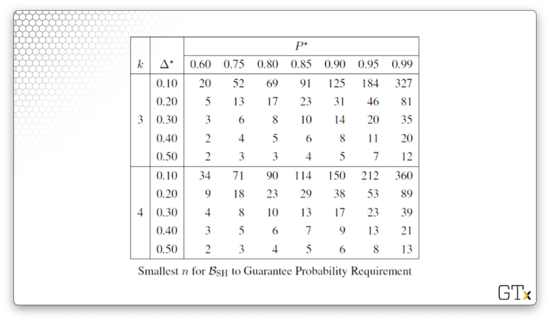
Let's look at the single-stage procedure, $\mathcal{B}_{\text{SH}}$, from Sobel and Huyett.

For specified $(P^*, \Delta^*)$, we find $n$ in the table. Here's the table:

Next, we take a sample of $n$ observations, $X_{ij} (1 \leq j \leq n)$, in a single stage from each population $(1 \leq i \leq k)$. From there, we calculate the $k$ sample sums:

In plain English, $Y_{in}$ represents the number of successes from the $i$th population under study. We then select the treatment that yielded the largest $Y_{in}$ as the one associated with $p_{[k]}$. If there happens to be a tie, we select a random winner among the ties.

Example

Suppose we want to select the best of $k = 4$ treatments. We want to be correct with probability of at least $P^* = 0.95$ whenever $p_{[4]} - p_{[3]} \geq 0.10$. The table shows that we need $n = 212$ observations from each population to meet this requirement.

Suppose that, at the end of sampling, we have the following success counts:

Then we select population two as best.

Bernoulli Extensions (OPTIONAL)

In this lesson, we will look at extensions of the Bernoulli procedure from the previous lesson. These extensions will save us many observations.

Curtailment

Let's look at a single-stage extension from Bechhofer and Kulkarni called curtailment. Here, we carry out the single-stage procedure, except we stop sampling when the population in second place can at best tie. It doesn't make sense to take any more observations after a winner is guaranteed.

As it turns out, curtailment gives the same probability of correct selection, $P(\text{CS})$, but with a lower expected number of observations, $x \leq n$.

For example, remember that, when $k=4$, $P^*=0.95$, and $\Delta^* = 0.10$, the single-stage procedure requires us to take $n = 212$ observations from each population, for a total of $N = 848$ observations.

Suppose that, after taking 180 samples from each population, we have the intermediate result $Y_{1,180} = 50$, $Y_{2,180} = 130$, $Y_{3,180} = 74$, and $Y_{4,180} = 97$.

We can stop sampling right now and select population two as the best because it's not possible for population four to catch up in the remaining $212 - 180 = 32$ observations. At best, $Y_{4,212} = 129 < Y_{2,180} \leq Y_{2,212}$.

A Sequential Procedure

An even better procedure is the sequential procedure, $\mathcal B_{\text{BKS}}$, by Bechhofer, Kiefer, and Sobel from 1968.

This procedure involves a new probability requirement. For specified $(P^*, \theta^*)$, with $1/k < P^* < 1$ and $\theta^* > 1$, we require $P(\text{CS}) \geq P^*$ whenever the odds ratio:

Here, we are taking the ratio of the odds that the $k$th population is the best over the odds that the $k-1$th population is the best. Whenever that ratio is $\geq \theta^*$, we want to ensure that the probability of correct selection is at least $P^*$.

The procedure proceeds in stages. We take one Bernoulli observation from each population, and we reevaluate to see if the odds ratio satisfies our requirement. This method is even more efficient than curtailment, which is more efficient than the basic single-stage procedure.

Let's take a look at the procedure itself. At the $m$th stage of experimentation, $m \geq 1$, we observe the random Bernoulli vector, $(X_{1m},...,X_{km})$. For example, if we are looking at $k = 5$ populations, the vector might look like $(0,1,1,1,0)$.

Next, we compute the population sums so far:

Then, we order the sums:

We stop at stage $m$ if the following inequality holds:

If the difference $Y_{[k]m} - Y_{[i]m}$ is large, for all $i$, then $1 / \theta^*$ raised to that power will be small, and the summation is likely to be less than $(1- P^*) / P^*$. In other words, we stop when the best population is sufficiently ahead of the remaining populations.

Let's let $N$ be the random stage $m$ when the procedure stops. Then, we select the population yielding $Y_{[k]N}$ as the one associated with $p_{[k]}$.

For example, let $k = 3$ and $(P^*, \theta^*) = (0.75, 2)$. Suppose we obtain the following sequence of vector-observations using $\mathcal B_{\text{BKS}}$:

Given $P^* = 0.75$, we stop when $Z_m \leq (1-0.75)/0.75 = 1/3$. After the $N = 6$ round of sampling, we get $Z_6 = 0.25 \leq 1/3$, and we choose the population with the largest $Y_{im}$ as the one associated with $p_{[k]}$. In this case, we choose population three.

Multinomial Cell Selection

In this lesson, we will talk about the multinomial selection problem, which corresponds to the problem of finding the most-probable category. This selection problem has applications in surveys, simulations, and more.

Multinomial Selection - Intro

We want to select the multinomial cell (category) having the largest probability. For example:

• Who is the most popular political candidate?
• Which television show is most-watched during a particular time slot?
• Which simulated warehouse configuration is most likely to maximize throughput?

These questions are different than the Bernoulli examples we looked at previously. In those examples, the populations succeeded or failed independently of one another. In this case, the various cells are competing against each other.

Yet again, we will take the indifference-zone approach, albeit in a slightly different way than in the binomial procedure.

Here's the experimental setup. We have $k$ possible outcomes. The probability that we will select a given category, $i$, as being the most probable is $p_i$. We will take $n$ independent replications of the experiment and let $Y_i$ equal the number of outcomes falling in category $i$ after taking the $n$ observations.

Let's look at a definition. Suppose we have a $k$-variate discrete vector random variable $\bold Y = (Y_1, Y_2,...,Y_k)$ with the following probability mass function:

If $Y$ has the probability mass function, then $\bold Y$ has the multinomial distribution with parameters $n$ and $\bold p = (p_1,...,p_k)$, where $\sum_{i=1}^k p_i = 1$ and $p_i > 0$ for all $i$. The multinomial generalizes the binomial.

Example

Suppose three of the faces of a fair die are red, two are blue, and one is violet. Therefore $\bold p = (3/6, 2/6, 1/6)$. Let's toss the die $n=5$ times. Then the probability of observing exactly three reds, no blues, and two violets is:

Now suppose that we did not know the probabilities for red, blue, and violet, and we want to select the most probable color. Using the selection rule, we choose the color the occurs the most frequently during the five trials, using randomization to break ties.

Let $\bold Y = (Y_r, Y_b, Y_v)$ denote the number of occurrences of (red, blue, violet) in five trials. The probability we correctly select red is:

Notice that we have a coefficient of 0.5 in front of the cases where red ties because we randomly break two-way ties, selecting each color with a probability of 0.5.

We can list the outcomes favorable to a correct selection of red, along with the associated probabilities (calculated using the multinomial pmf above), randomizing in case of ties:

As we can see, in this case, the probability of correct selection is 0.6042, given $n=5$ observations. We can increase the probability of correct selection by increasing $n$.

Example 2

The most probable alternative might be preferable to that having the largest expected value. Consider two inventory policies, $A$ and $B$. The profit from $A$ is $5 with probability one, and the profit from $B$ is $0 with probability 0.99 and $1000 with probability 0.01.

The expected profit from $A$ is $5 and the expected profit from $B$ is $10: $1000 * 0.01 + 0 = 10$. However, the actual profit from $A$ is better than the profit from $B$ with probability 0.99. Even $E[A] < E[B]$, $A$ wins almost all of the time.

Multinomial Procedure & Extensions

In this lesson, we'll look at the single-stage procedure for selecting the most-probable cell along with a few extensions.

Assumptions and Notation for Selection Problem

Let's let $\bold X_j = (X_{1j},...,X_{kj}), \enspace j \geq 1$ be independent observations taken from a multinomial distribution having $k \geq 2$ categories with associated unknown probabilities $\bold p = (p_1,...,p_k)$.

For a fixed $j$, $X_j$ refers to one multinomial observation, which is of length $k$, corresponding to each of the $k$ categories. For example, if we have $k=8$ political candidates to choose from, $X_j$ has $k=8$ entries.

The entry $X_{ij}$ equals one if category $i$ occurs on the $j$th observation. Otherwise, $X_{ij} = 0$. For example, if we ask someone to choose from eight different candidates, and they choose candidate one, then $X_{1j} = 1$ and $X_{2j} = \cdots = \ X_{8j} = 0$.

We can order the underlying, unknown $p_i$'s like so: $p_{[1]} \leq \cdots \leq p_{[k]}$. The category with $p_{[k]}$ is the most probable or best category.

We will survey many people and count up the number of times they select each category. The cumulative sum for category $i$ after we take $m$ multinomial observations is:

The ordered $Y_{im}$'s are $Y_{[1]m} \leq \cdots \leq Y_{[k]m}$. We select the candidate associated with $Y_{[k]m}$ as being associated with $p_{[k]}$.

Our goal in this problem is to select the category associated with $p_{[k]}$, and we say that a correct selection is made if the goal is achieved. For specified $(P^*, \theta^*)$, where $1/k < P^* < 1$ and $\theta^* > 1$, we have the following probability requirement:

When the ratio of the best category to the second-best category eclipses a certain $\theta^*$ that we specify, we want to ensure that we make the right selection with at least probability $P^*$. We can interpret $\theta^*$ as the smallest $p_{[k]} / p_{[k-1]}$ ratio worth detecting.

Single-Stage Procedure

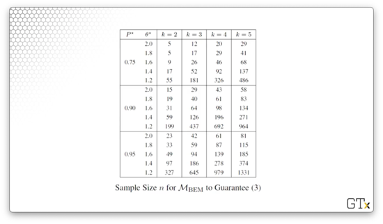
Let's look at the single-stage procedure, $\mathcal M_{\text{BEM}}$, by Bechhofer, Elmaghraby, and Morse, from 1959. For a given $k$, $P^*$, and $\theta^*$, we find the required number of multinomial observations, $n$, from a table.

First, we take $n$ multinomial observations $(X_{1j},...,X_{kj}) \enspace 1 \leq j \leq n$ in a single stage. From there, we calculate the ordered sample sums, $Y_{[1]n} \leq \cdots \leq Y_{[k]n}$. Finally, we take the category with the largest sum, $Y_{[k]n}$ as the one associated with $p_{[k]}$, randomizing to break ties.

The $n$-values are computed so that $\mathcal M_{\text{BEM}}$ achieves $P(\text{CS}) \geq P^*$ when the cell probabilities $\bold p$ are in the least-favorable configuration:

In this configuration, the best category is ahead of all of the other categories by a factor of exactly $\theta$, and the other $p_i$'s are all identical.

In any event, here is the table, parameterized by $k$, $P^*$, and $\theta^*$ that guarantees the appropriate probability of correct selection.

Example

A soft drink producer wants to find the most popular of $k=3$ proposed cola formulations. The company will give a taste test to $n$ people. The sample size $n$ is to be chosen so that $P(\text{CS}) \geq 0.95$ whenever the ratio of the largest to second largest true (but unknown) proportions is at least 1.4.

From the table, we see that, for $k=3$, $P^* = 0.95$, and $\theta^* = 1.4$, we need to take $n = 186$ multinomial observations. Let's take those observations and assume that we find $Y_{1,186} = 53$, $Y_{2,186} = 110$, and $Y_{3,186 = 26}$. Then, we select formulation two as the best.

Extensions

We can use curtailment in multinomial cell selection and stop sampling when the category in second place cannot win. Additionally, we can use a sequential procedure and take observations one at a time until the winner is clear.