Applications Videos

Multimedia Applications: A Perspecitve From the Network

So why are we choosing to talk about multimedia applications?

Most undergraduate networking courses discuss some of the more traditional network applications, such as email or web browsing. In this course, we wanted to expose you to some of the more interesting and rapidly evolving network applications. In this lesson, we will be discussing multimedia applications, which are defined in Kurose and Ross as “any network application that employs audio or video.” These applications deal with different challenges, with interesting techniques for addressing those challenges.

For example, when users are streaming video, they expect the video to play back with the same timing that it was originally recorded - which means users expect that it won't randomly speed up or freeze while they are watching - and this can be addressed with buffering techniques. Or for another example, users in a VoIP conference call expect to hear each other's voices relatively quickly - a one second delay can be very frustrating and make people accidentally talk over each other.

Each type of multimedia application has different requirements, and thus, different challenges and techniques for addressing those challenges.

Background: Video and Audio Characteristics

Before we talk about different kinds of multimedia applications, such as streaming video, let's take a moment to discuss some basic video and audio properties. This will give us some context for some of our later discussions, such as how bitrate adaption algorithms work.

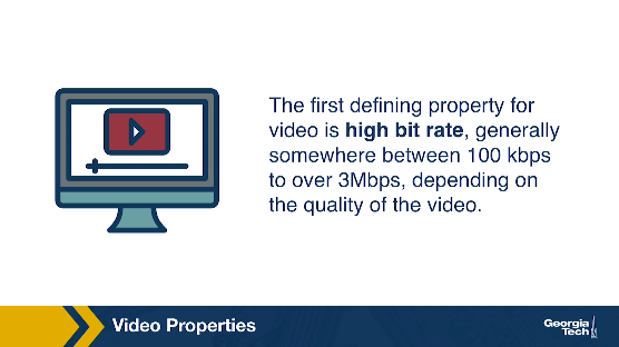
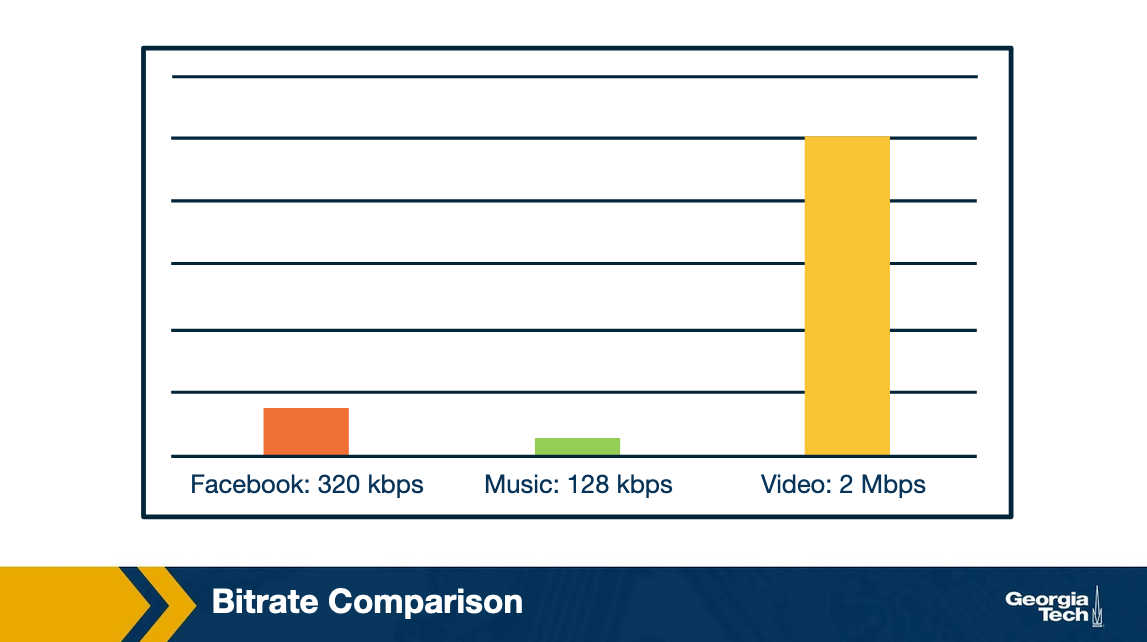
First, let's talk about video. The first defining property for video is high bit rate, generally somewhere between 100 kbps to over 3Mbps, depending on the quality of the video. For perspective on just how much higher video bitrates are than browsing through an online photo gallery or listening to streaming music, here is a somewhat typical example. If the Facebook user is flipping through a photo gallery at about one photo every 5 seconds, typical rates would look something like this:

However, there are techniques for compressing video, with varying levels of compression and video quality. We will be discussing some of these techniques later in the lesson.

Now, let's take a moment to also talk about audio. Audio has a lower bit rate than video, as we already mentioned, but glitches in audio are generally more noticeable than glitches in video. For example, in a video conference, it's generally ok if the video cuts out or freezes for a few seconds here and there, but if the audio also cuts out or gets garbled, you'd probably end up having to cancel or reschedule the conference.

Also, like video, audio can be compressed at varying quality levels.

Types of Multimedia Applications and Characteristics

The different kinds of multimedia applications can be organized into three major categories. There's (a) streaming stored audio and video, such video clips on Udacity for our OMSCS courses, (b) conversational voice and video over IP, such as Skype, and (c) streaming live audio and video, such as the graduation ceremony for GATech on graduation day. Let's discuss some of the characteristics for each of these three categories.

First, streaming stored video is...streamed! That means that the video starts playing within a few seconds of receiving data, instead of waiting for the entire file to download first. It's also interactive, which means that the user can pause, fast forward, skip ahead or move back in the video, and then see the response within a few seconds. Streaming stored video should also have continuous playout, which means that it should play out the same way it was recorded without freezing up in the middle. Generally, streaming stored video files are stored on a CDN rather than just one data center. This type of multimedia application can also be implemented with the peer-to-peer model instead of the client-server model.

Streaming live audio and video is very similar to streaming stored video or audio, and use similar techniques, with some important differences. Since these applications are live and broadcast-like, there are generally many simultaneous users, sometimes in very different geographic locations. They are also delay-sensitive, but not as much as conversational voice and video applications are - generally, a ten second delay is ok. We'll also be discussing these applications in more detail later in the lesson.

Second, let's talk about conversational voice and video over IP. Notice that VoIP stands for “Voice over IP”, which is like phone service that goes over the Internet instead of through traditional circuit-switched telephony network. These kinds of calls or video conferences often involve three or more participants. Since these calls and conferences are real-time and involve human users interacting, these applications are highly delay-sensitive. A short delay of less than 150 milliseconds isn't really noticeable, but a longer delay, such as over 400 milliseconds, can be frustrating as people end up accidentally talking over each other. On the other hand, these applications are loss-tolerant. There are techniques that can conceal occasional glitches, and even if a word in the conversation gets garbled, human listeners are generally able to ask the other side to just repeat themselves.

How Does VoIP Work?

Let's take a closer look at VoIP, which falls in the category of “conversational voice over IP.” We will focus on conversational audio, although video that works in similar ways.

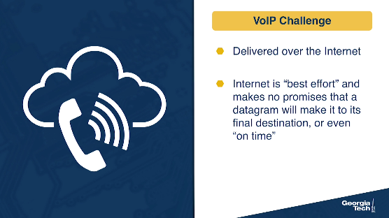
VoIP has the challenge that it is transmitted over the Internet. Since the Internet is “best effort” and makes no promises that a datagram will actually make it to its final destination, or even “on time,” this is no small challenge for VoIP! In this topic, we'll discuss three major topics in VoIP, which are also applicable to other multimedia applications to varying degrees: encoding, signaling, and QoS (Quality of Service) metrics.

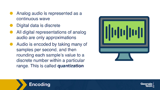
First, let's talk about how the analog audio gets encoded into a digital format, and how that impacts VoIP. Analog audio by nature is represented as a continuous wave, but digital data by nature is discrete. Therefore, all digital representations of analog audio are only approximations. Generally speaking, audio is encoded by taking many (as in, thousands) of samples per second, and then rounding each sample's value to a discrete number within a particular range. (This “rounding” to a discrete number is called quantization.)

Example technique: For example, PCM (Pulse Code Modulation) is one technique used with speech, taking 8000 samples per second, and with each sample's value being 8 bits long. On the other hand, PCM with an audio CD takes 44,100 samples per second, with each sample value being 16 bits long. You can see how with more samples per second, or a larger range of quantization values, the digital approximation gets closer to the actual analog signal, which means a higher quality when playing it back. But the tradeoff is that it takes more bits per second to play back the audio.

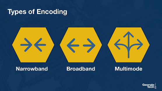
Encoding schemes: The three major categories of encoding schemes are narrowband, broadband, and multimode (which can operate on either), and they come with different characteristics and tradeoffs. For VoIP, the important thing is that we want to still be able to understand the speech and the words that are being said, while at the same time still using as little bandwidth as possible.

As a final note on this topic, audio can also be compressed, but there are some tradeoffs there too. We'll be discussing video compression techniques later in this lesson when we talk about streaming video, and many of those concepts (such as how packet loss can greatly interfere with some compression techniques) also apply to audio compression.

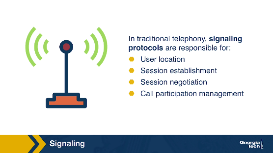
Second, let's talk about signaling. In traditional telephony, a signaling protocol takes care of how calls are set up and torn down. Signaling protocols are responsible for four major functions. 1) User location - the caller locating where the callee is. 2) Session establishment - handling the callee accepting, rejecting, or redirecting a call. 3) Session negotiation - the endpoints synchronizing with each other on a set of properties for the session. 4) Call participation management - handling endpoints joining or leaving an existing session.

VoIP also uses signaling protocols, just like telephony, to perform the same functions. The SIP (Session Initiation Protocol) is just one example of a signaling protocol used in many VoIP applications.

QoS for VoIP: Metrics

Now let's talk about the QoS metrics - that is, how we measure the quality of service. There are three major QoS metrics for VoIP:

• end-to-end delay
• jitter
• packet loss

Let's talk about these in more detail, and why they're so important to VoIP applications.

QoS for VoIP: End-to-End Delay

Our first QoS metric is “end-to-end delay”, which is basically the total delay “from mouth to ear.” This includes delay from:

• the time it takes to encode the audio (which we discussed earlier),
• the time it takes to put it in packets,
• all the normal sources of network delay that network traffic encounters such as queueing delays,
• “playback delay,” which comes from the receiver's playback buffer (which is a mitigation technique for delay jitter, which we'll be discussing next),
• and decoding delay, which is the time it takes to reconstruct the signal.

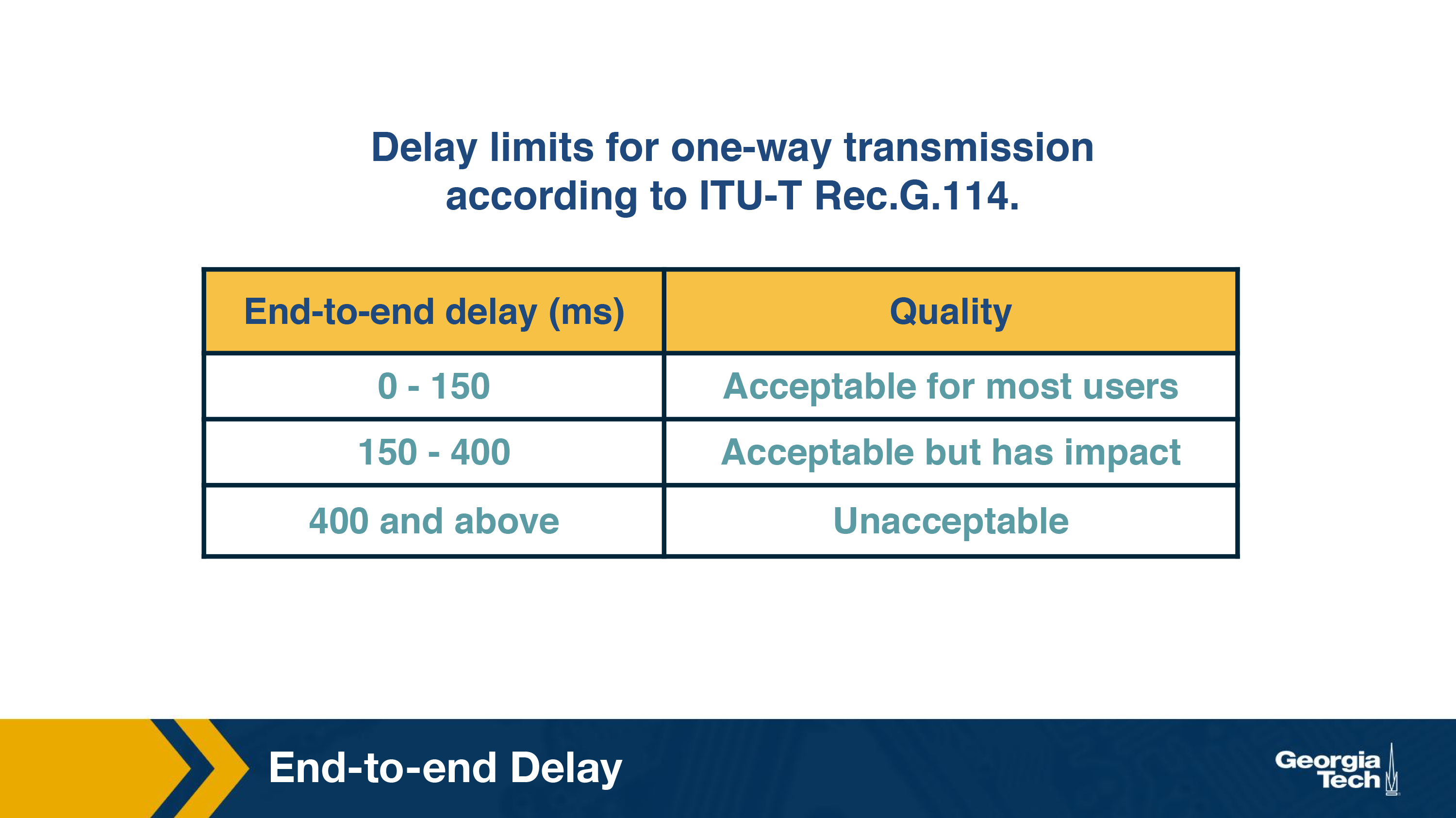
End-to-end delay is the accumulation of all of these sources of delay, and VoIP applications are sensitive to these delays. In general, an end-to-end delay of below 150ms is not noticeable by human listeners. A delay between 150ms and 400ms is noticeable, but perhaps acceptable, depending on the purpose of the VoIP call and the human users' expectations (we might be more accepting of delays if we are calling a more remote region, for instance). However, an end-to-end delay greater than 400ms starts becoming unacceptable, as people start accidentally talking over each other.

Since delays are so impactful for VoIP, VoIP applications frequently have delay thresholds, such as at 400ms, and discard any received packets with a delay greater than that threshold. That means that packets that are delayed by more than the threshold are effectively lost.

QoS for VoIP: Delay Jitter

As you've learned in previous lessons for this class, between all the different buffer sizes and queueing delays and network congestion levels that a packet might experience, different voice packets can end up with different amounts of delay. One voice packet may be delayed by 100ms, and another by 300ms. We call this phenomenon “jitter,” “packet jitter,” or “delay jitter.”

It turns out that jitter is problematic for VoIP, because it interferes with reconstructing the analog voice stream. With large jitter, we end up with more delayed packets that end up getting discarded, and that can lead to a gap in the audio. Too many dropped sequential packets can make the audio unintelligible. Because the human ear is pretty intolerant of audio gaps, audio gaps should ideally be kept below 30ms, but depending on the type of voice codec used and other factors, audio gaps between 30 to 75ms can be acceptable.

The main VoIP application mechanism for mitigating jitter is maintaining a buffer, called the “jitter buffer” or the “play-out buffer.” This mechanism helps to smooth out and hide the variation in delay between different received packets, by buffering them and playing them out for decoding at a steady rate. There's a tradeoff here, though. A longer jitter buffer reduces the number of packets that are discarded because they were received too late, but that adds to the end-to-end delay. A shorter jitter buffer will not add to the end-to-end delay as much, but that can lead to more dropped packets, which reduces the speech quality.

QoS for VoIP: Packet Loss

Our last QoS metric to discuss is the ratio of packet loss.

Packet loss is pretty much inevitable - after all, VoIP operates on the Internet, and the Internet is a “best-effort” service. VoIP protocols could use TCP, since TCP eliminates packet loss by retransmission, but the problem is that TCP does that by retransmitting lost packets, and as we discussed earlier, those retransmitted packets are no good if they are received too late. Plus, TCP congestion control algorithms drop the sender's transmission rate every time there's a dropped packet, and we can end up with the sender dropping the transmission rate lower than the receiver's drain rate from playing out the audio. So most of the time, VoIP protocols use UDP.

What we consider packet loss for VoIP. So, we end up with a different definition for packet loss. With VoIP, a packet is lost if it either never arrives OR if it arrives after its scheduled playout. This is a harsher definition than for other applications (such as file transfers), but thankfully, VoIP can tolerate loss rates of between 1 and 20 percent, depending on what voice codec is used and other factors.

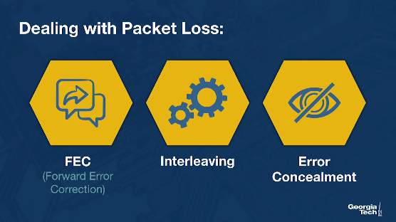
VoIP protocols have three major methods of dealing with packet loss: FEC (Forward Error Correction), interleaving, and error concealment.

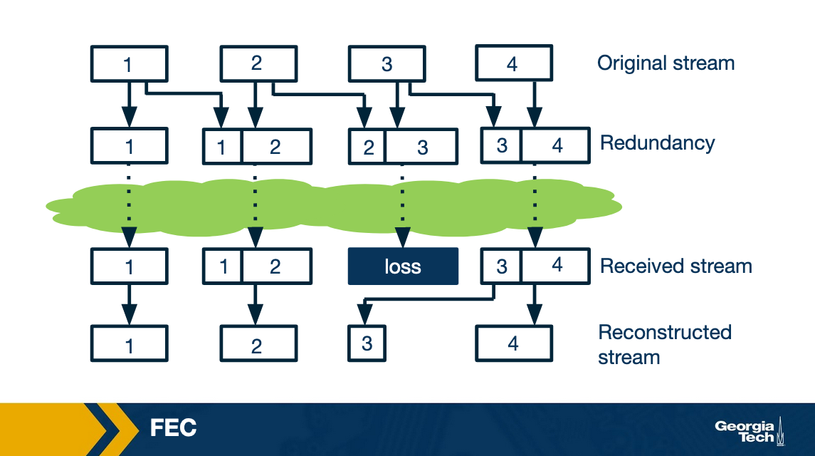
FEC (Forward Error Concealment) comes in a few different flavors, but in general, FEC works by transmitting redundant data alongside the main transmission, which allows the receiver to replace lost data with the redundant data. This redundant data could be a copy of the original data, by breaking the audio into chunks and cleverly using exclusive OR (XOR) with n previous chunks. This redundant data could also be a lower-quality audio stream transmitted alongside the original stream - similar to how a spare tire in a car may be of lower quality than the normal tires, but enough to get by in the case of a flat tire. Regardless of which method is used, there's a tradeoff.

The more redundant data transmitted, the more bandwidth is consumed. Also, some of these FEC techniques require the receiving end to receive more chunks before playing out the audio, and that increases playout delay.

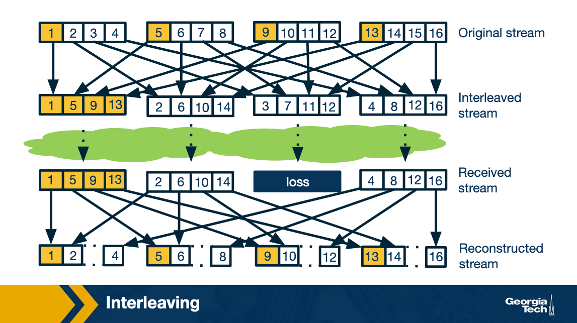
Interleaving, on the other hand, interleaving does not transmit ANY redundant data, and so it doesn't add extra bandwidth requirements or bandwidth overhead. Interleaving works by mixing chunks of audio together so that if one set of chunks is lost, the lost chunks aren't consecutive. The idea is that many smaller audio gaps are preferable to one large audio gap. (We note that the human ear is pretty intolerant of audio gaps, and ideally audio gaps should be under 30ms.)

The tradeoff for interleaving is that the receiving side has to wait longer to receive consecutive chunks of audio, and that increases latency. Unfortunately, that means this technique is limited in usefulness for VoIP, although it can have good performance for streaming stored audio.

The last technique for dealing with packet loss, error concealment, is basically “guessing” what the lost audio packet might be. This is possible because generally, with really small audio snippets (like between 4ms and 40 ms), there's some similarity between one audio snippet and the next audio snippet. This is the same principle that makes audio compression possible.

One really simple version of error concealment is to simply repeat a packet - replace the lost packet with a copy of the previous packet - and hope that will be good enough. This solution is computationally cheap, and works pretty well in a lot of cases. Another version of error concealment is to use the audio before and after the lost packet and interpolate (that is, make a calculation to guess) an appropriate packet to conceal the lost packet. This is a better solution than packet repetition, but it is more computationally expensive.

Live/On Demand Streaming Introduction

So far we looked at how real-time interactive streaming worked. We will now study the mechanisms behind streaming media content over the Internet, which accounts for nearly 60-70% of the Internet traffic. Various enabling technologies and trends have led to this development of consuming median content over the Internet. One, the bandwidth for both the core network and last-mile access links have increased tremendously over the years. Two, the video compression technologies have become more efficient. This enables to stream high-quality video without using a lot of bandwidth. Finally, the development of Digital Rights Management culture has encouraged content providers to put their content on the Internet.

The types of content that is streamed over the Internet can be divided into two categories: i) Live -- this means the video content is created and delivered to the clients simultaneously. Examples can be streaming of sports events, music concerts etc, and ii) On-demand -- this includes streaming stored video based on users' convenience. Examples can be watching videos on Netflix, non-live videos on YouTube etc. As you can imagine, the constraints for streaming live and on-demand content differ slightly. One of the main constraints being that there is not a lot of room for pre-fetching content in the case of live streaming. In this lesson, we will focus mainly on understanding streaming of the on-demand video. It turns out that most of the basic principles behind streaming live at large-scale and on-demand content are similar apart from the few details such as video encoding.

Video Streaming Bigger Picture

Let's begin with a high-level overview of how streaming works. Here is a figure showing the different steps involved in video streaming.

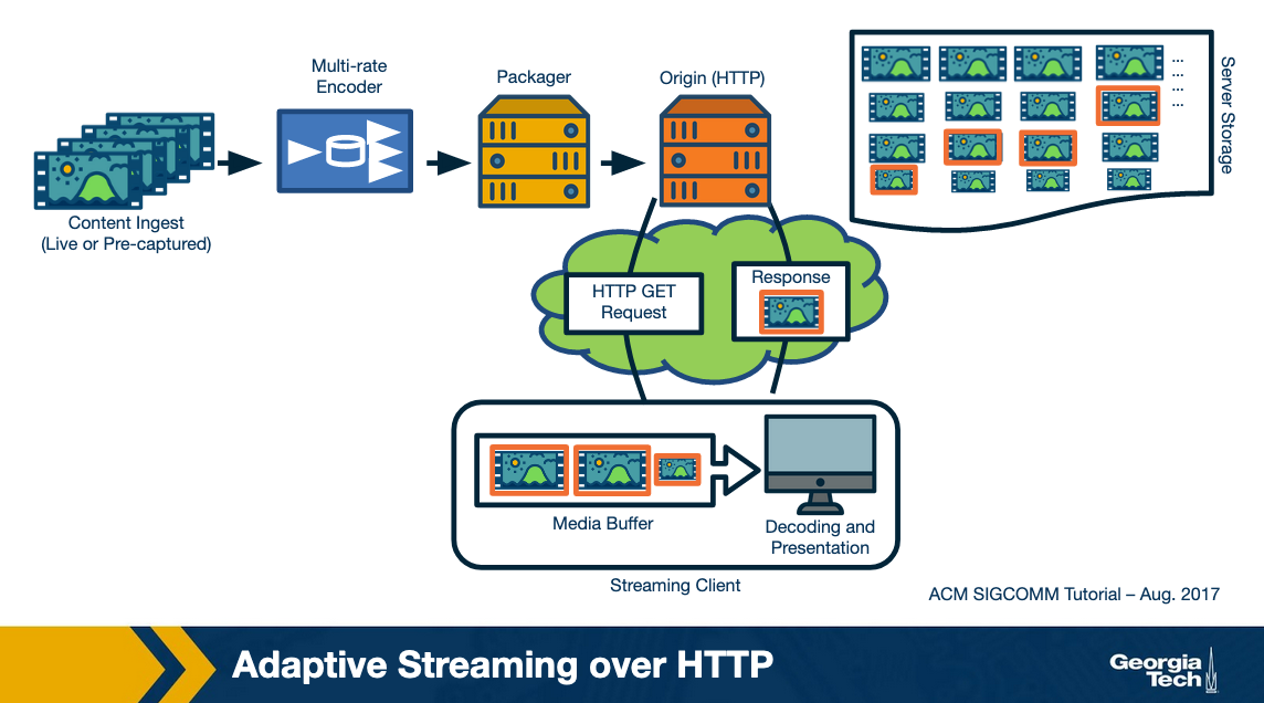
The video content is first created -- say in a professional studio like this lesson or using a smartphone by a user. The raw recorded content is typically at a high quality. It is then compressed using an encoding algorithm. This encoded content is then secured using DRM and hosted over a server. Typically content providers have their own data centers such as Google or use third-party Content delivery networks to replicate the content over multiple geographically distributed servers. This makes sure that the content can be delivered in a scalable manner. The end-users download the video content over the Internet. The downloaded video is decoded and rendered on the user's screen.

In the remaining lesson, we will delve deeper into these steps. We will answer questions like how does the video compression work? What application and transport-layer protocols are used for video delivery? How do we ensure that the same content can be watched under a diversity of network conditions and using different user devices?

Sources of Redundancy in Video Compression

We will start with looking at how video compression works. Video compression essentially consists of reducing the size of the video by compressing it. The compression can be of two types -- lossy, in which we can not recover the high quality video and loss-less, in which the original video can be recovered. It is intuitive that lossy compression gives higher savings in terms of bandwidth and hence that is what is used by video compression algorithms these days.

Let us understand how this works. The goal of a compression algorithm is to cut down data by removing “similar” information from the video while not compromising a lot with the video quality. Now, what could be the potential sources of “similarity” in a video?

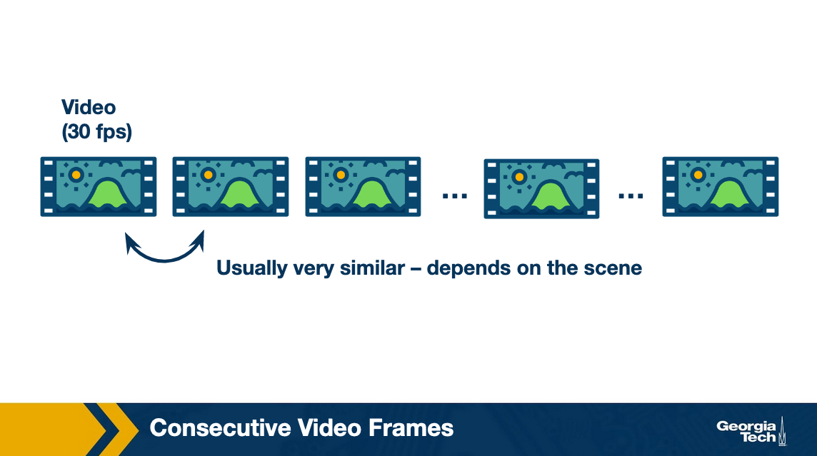
If we consider a video, it is essentially a sequence of digital pictures, where each picture is a 2-D sequence of pixels. An efficient compression can be achieved in two-ways: i) within an image -- pixels that are nearby in a picture tend to be similar -- known as spatial redundancy, and ii) across images -- in a continuous scene, consecutive pictures are similar -- known as temporal redundancy. Let us look at each of these components in detail.

Image Compression

For the first component, aka image compression, let's look at the steps that take place.

The Joint Photographics Experts Group (JPEG) standard, was developed. The main idea behind JPEG is how to represent an image using components that can be further compressed.

It essentially consists of four steps:

Step 1

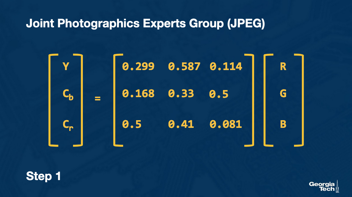
Let us assume that we are given an RGB image of 640*480. The first step is to transform it into color component (chrominance or Cb, Cr) and brightness component (luminance or Y). This is done because human eyes are more sensitive to brightness and at the same time we could further compress Cb and Cr. Now our image is represented with 3 matrices: Y, Cb, Cr.

We obtain the 3 matrices Y, Cb and Cr from RGB by using the conversion below:

Step 2

We operate on of each of these three matrices (Y Cb Cr) independently. We compress and encode them separately. For each of the 3 matrices we perform the same steps we describe next.

We divide the image into 8x8 blocks (sub-image). We apply the Discrete Cosine Transformation to each of the sub-images to transform it into the frequency domain. The output (for each sub-image) is an 8x8 table of DCT coefficients, with each element representing the spectral power (weight) present at that spatial frequency.

This is done because the human eye is less sensitive to high-frequency coefficients as compared to low-frequency coefficients. Thus, the latter can be compressed significantly using quantization.

Step 3

In this step (this is the lossy step of the process), we compress the matrix of the coefficients using a pre-defined Quantization table (Q).

Fquantized(u, v) = F(u, v) / Q(u, v)

Each entry of the coefficient table is divided by the corresponding entry in the quantization table (and then it is rounded to the nearest integer). Note that the weights are higher for higher spectral frequencies. Also, the degree of quantization impacts the quality of the image. Thus, based on the desired image quality, different levels of quantizations can be performed. Also, the Quantization table is stored in the image header so the image can be later decoded.

Step 4

Once we obtain the quantized matrices for each of the 8*8 block in the image, we perform a lossless encoding to store the coefficients. The details of this are given in an optional reading. This finishes the encoding process.

This encoded image is then transferred over the network and is decoded at the user-end.

Video Compression and Temporal Redundancy

So far, we looked at how a frame in the video is compressed. Can we do better? Well, consecutive frames in a video are similar to each other.

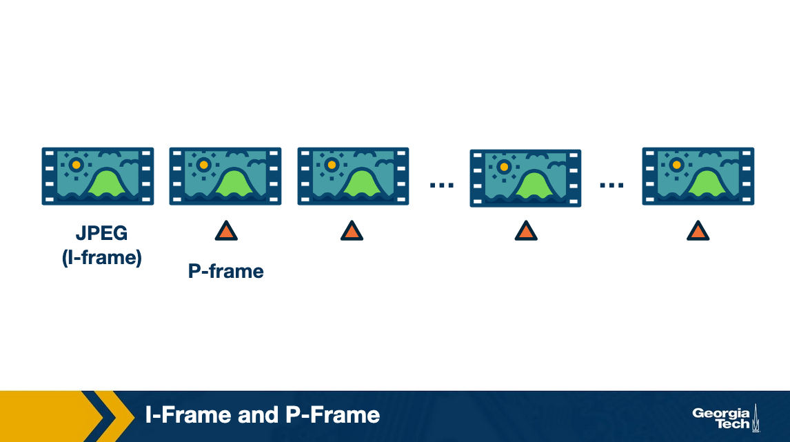
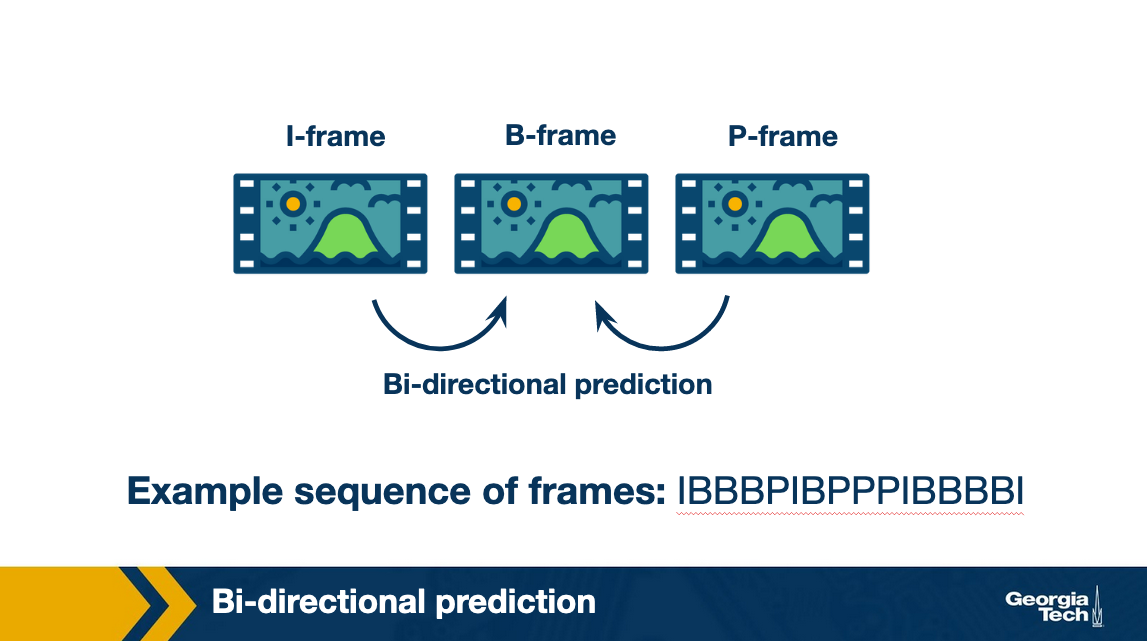
Thus, instead of encoding every image as a JPEG, we encode the first (known as I-frame) as a JPEG and then encode the difference between two frames. The in-between encoded frame is known as Predicted or P-frame.

Note that, we do not want to use the difference all the way. This is because of two reasons:

1. When a scene changes, the frame becomes drastically different from the last frame and even if we are using the difference, it is almost like encoding a fresh image. This can lead to loss in image quality.
2. In addition, it also increases the decoding time in case a user skips ahead in the video as it will need to download all frames in between the last I-frame and the current frame to decode the video.

Thus a typical solution is to insert an I-frame periodically, say after every 15 frames. All the frames between two consecutive I-frames is known as a Group of Pictures (GoP).

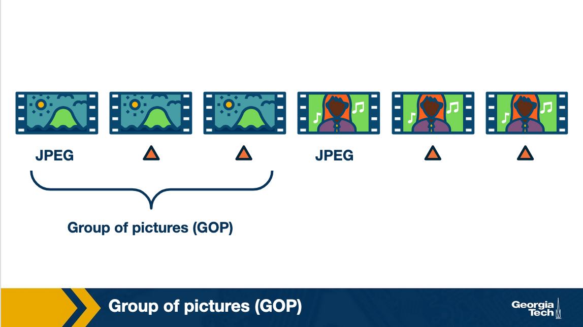
An additional way to improve encoding efficiency is to encode a frame as a function of the past and the future I (or P)-frames. Such a frame is known as a Bi-directional or B-frame.

VBR vs CBR

Thus, we saw the basic mechanisms behind video compression algorithms. You might have realized that these algorithms provide knobs to control the trade-offs between the output image quality and its size. There are two ways to use these knobs for encoding videos.

In the first way, the output size of the video is fixed over time. This is known as constant bitrate encoding. In the second method, the output size remains the same on an average, but varies here and there based on the underlying scene complexity. This is known as variable bitrate encoding.

As you can imagine, the image quality is better in VBR as compared to CBR for the same bitrate. However, VBR is more computationally expensive as compared to CBR. You should note that video compression in general requires heavy-computation. In fact, for live streaming, wherein the video compression has to be done real-time, specialized (but expensive) hardware encoders are used by content providers.

UDP vs TCP

We have seen how compression works. The compressed video is stored in a server and is ready for delivery to the client over the network.

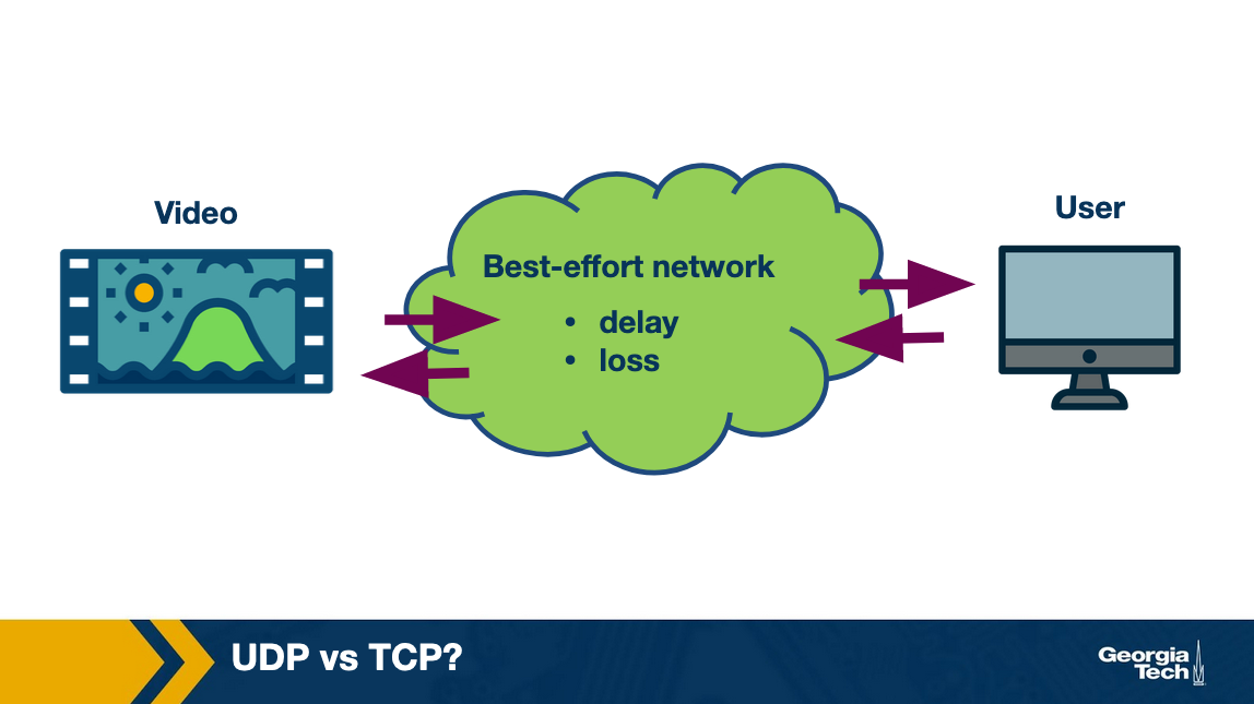
Let us think about what will be a good transport protocol to deliver. Note that the video needs to be decoded at the client. This decoding might fail if some data is lost. For instance, if an I-frame is lost partially, we may not be able to obtain the RGB matrices correctly. Similarly, if an I-frame was lost, P-frame can not be decoded. Therefore, we need a transport protocol that ensures that the data is delivered reliably over the Internet which is a best-effort network.

Thus, between UDP and TCP, content providers ended up choosing TCP for video delivery as it provides reliability. An additional benefit of using TCP was that it already provides congestion control which is required for effectively sharing bandwidth over the Internet.

Why Do We Use HTTP?

The next question we need to answer is what application-layer protocol be used for video delivery?

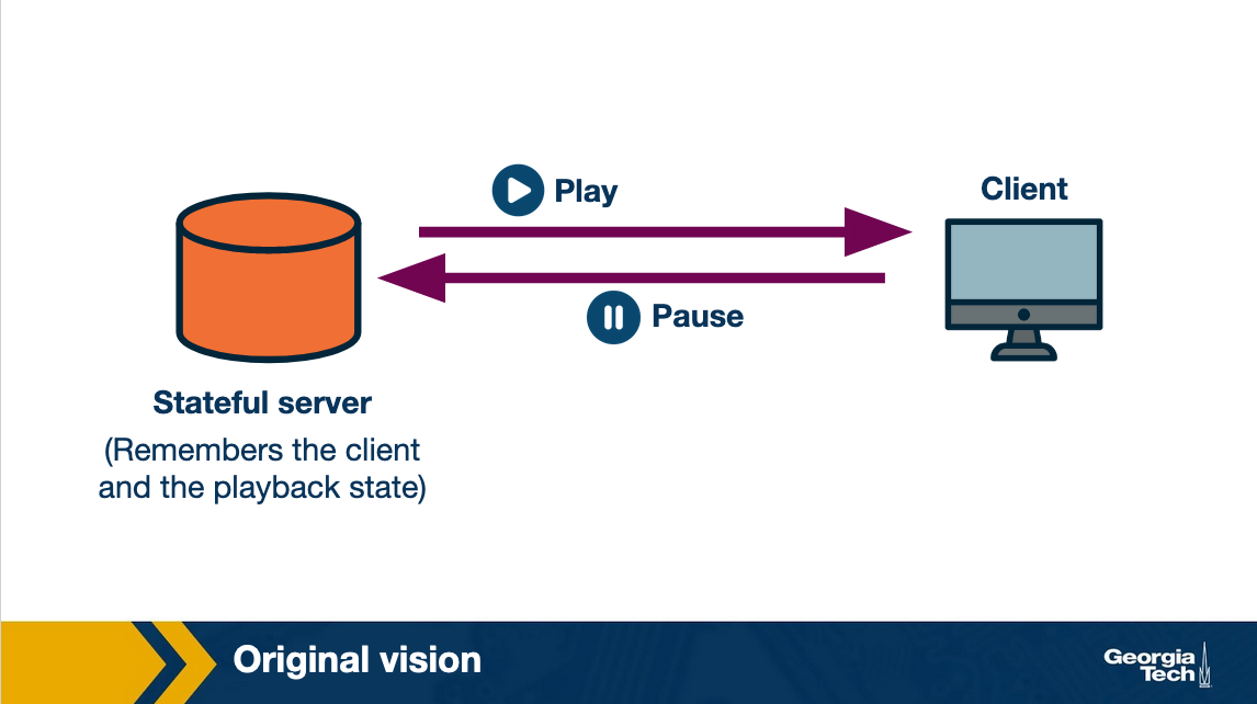
The original vision was to have specialized video servers that remembered the state of the clients. These servers would control the sending rate to the client. In the case, client paused the video, it would send a signal to the server and the server would stop sending video. Thus, all the intelligence would be stored at a centralized point and the clients, which can be quite diverse, would have to do minimal amount of work.

However, all this required content providers to buy specialized hardware.

Another option was to use the already existing HTTP protocol. In this case, the server is essentially stateless and the intelligence to download the video will be stored at the client. A major advantage of this is that content providers could use the already existing CDN infrastructure. Moreover, it also made bypassing middleboxes and firewalls easier as they already understood HTTP.

Because of the above advantages, the original vision was abandoned and content providers ended up using HTTP for video delivery.

Progressive Download vs Streaming

So far we have seen that the video is encoded and stored in an HTTP server.

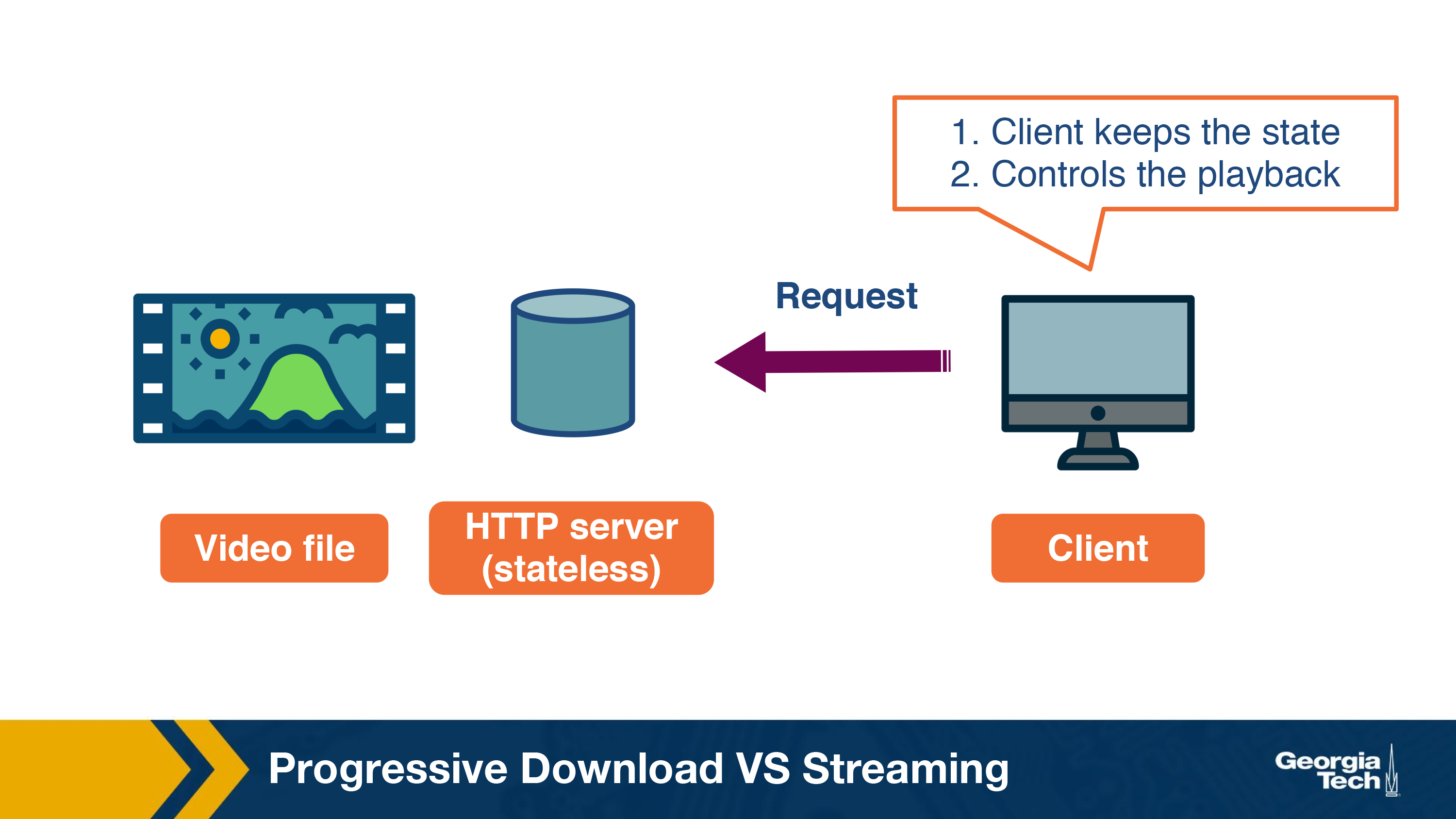
Given that the server is stateless, all the intelligence to stream the video would lie at the client-side. Let us now look at how the client fetches the video.

One way to stream the video would be to send an HTTP GET request for video. It is essentially like downloading a file over HTTP. The server will send the data as fast as possible, with the download rate limited only by the TCP rate control mechanisms. While quite simple, this has some disadvantages:

1. Users often leave the video mid-way. Thus, downloading the entire file can lead to a waste of network resources.
2. The video content that has been downloaded but not played so far would have to be stored. Thus, we will need a video buffer at the client to store this content in memory. This can be an issue particularly with long videos as large buffer would be required to store the content.

Thus, instead of downloading the content all at once, the client tries to pace it. This can be done by sending byte-range requests for part of the video instead of requesting the entire video. Once the video content has been watched, it sends request for more content. Ideally, this should be enough for streaming without stalls.

Thus, downloading video content over the Internet takes time which depends on the network throughput. We know that Internet is best-effort and throughput over the Internet is variable. This can lead to unnecessary stalling if the client is doing pure streaming i.e. downloading the video content just before it is to be played.

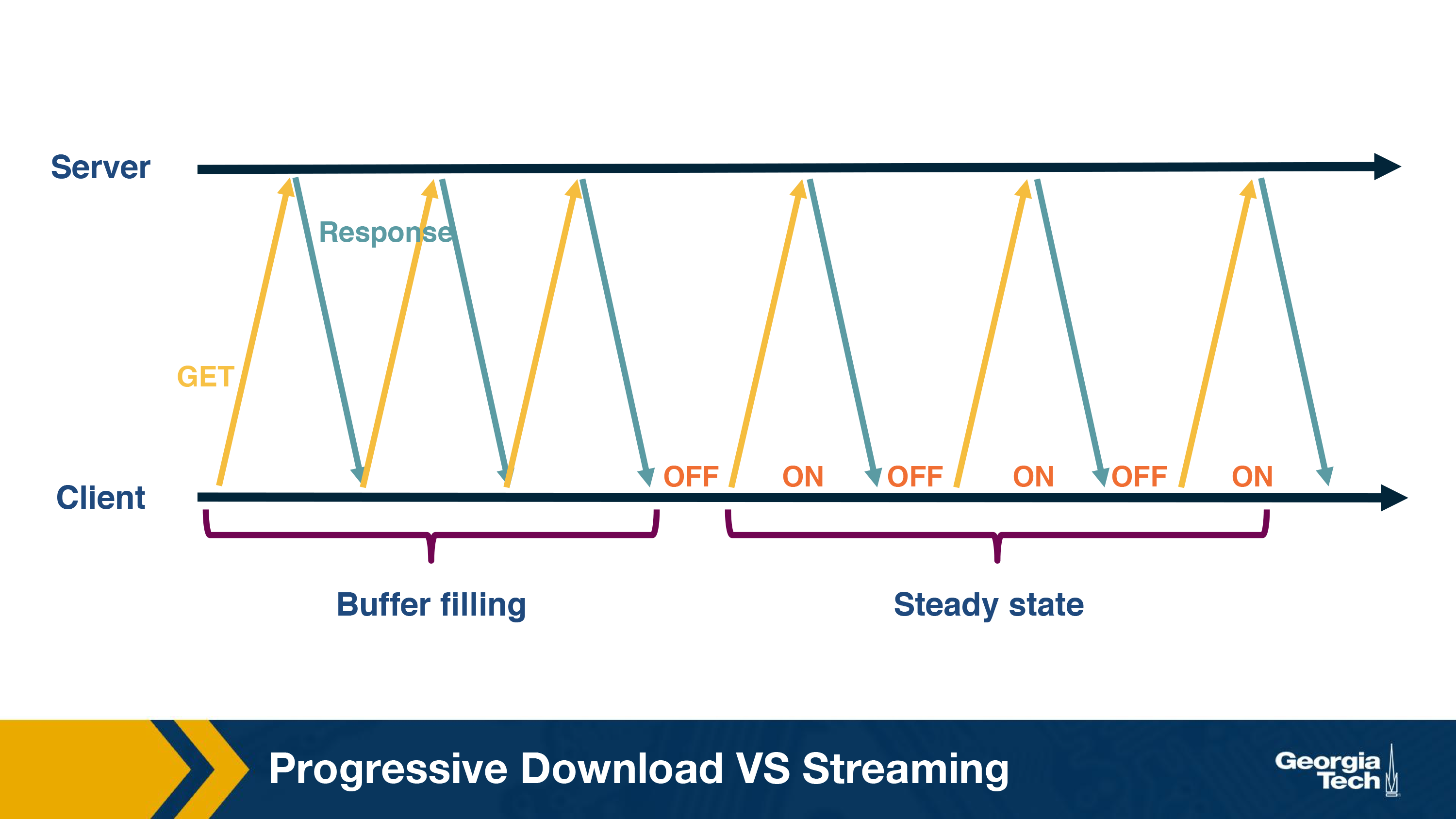
To account for these variations, client pre-fetches some video ahead and stores it in a playout buffer. The playout buffer is usually defined in terms of number of seconds of video that can be downloaded in advance or in terms of size in bytes. For example, the video buffer can be 5 seconds. Once, the video buffer becomes full, the client will wait for it to get depleted before asking for more content. Streaming in this manner typically has two states:

1. Filling state: This happens when the video buffer is empty and the client tries to fill it as soon as possible. For instance, in the beginning of the playback, the client tries to download as fast as possible until the buffer becomes full.
2. Steady state: After the buffer has become full, the client waits for it to become lower than a threshold. After which, the client sends a request for more content. The steady state is characterized by these ON-OFF patterns.

How to Handle Network and User Device Diversity?

It is important to note that a client's streaming context can be quite diverse. For example, the device over which you watch your favorite Netflix show varies, from a small screen smartphone to a large-screen TV. A low bitrate looks that looks good on a smartphone may not look that great over the TV.

Similarly, the network environments over which video streaming happens can be quite diverse. For instance, some of you might be watching this lesson over a fixed connection or over a WiFi access point where the Internet speed is high while others might be watching it over a cellular connection or a spotty Internet connection. A high bitrate video can be streamed seamless over a high-speed connection but not so without stalls over a spotty Internet connection.

To add to it, the Internet throughput can be quite transient. Let us consider a simple scenario, where you have 2 Mbps speed provided by your Internet provider. Say you are watching a Star Trek video encoded at 1.5 Mbps over this connection. Suddenly, one of your family members starts downloading a file over the same connection. Now your available bandwidth reduces to 1 Mbps and there is no way you would be able to watch the video without stalls, leading to a degradation in your streaming experience.

Thus, it is clear that a single-bitrate encoded video is not the best solution given the diversity in streaming context. Instead, content providers encode their video at multiple bitrates chosen from a set of pre-defined bitrates. Specifically, the video is chunked into segments which are usually of equal duration. Each of these segments is then encoded at multiple bitrates and stored at the server. The client request while requesting for a segment also specifies its quality.

For instance, the Star Trek episode could be divided into segments of 5s with each segment encoded at 250kbps, 500 kbps, 1.5 Mbps, 3Mbps, and 6 Mbps. Note that a higher bitrate usually leads to higher video quality. Now, consider the same scenario as before, when you are watching the video over a 2 Mbps connection. To get the best possible quality, you could stream the video at 1.5 Mbps. Once the available bandwidth reduces due to a background download, you can reduce the video quality and stream the video at 500 kbps, thus avoiding any stalls. When the background download is finished and your available throughput again becomes 2 Mbps, you can again start streaming at 1.5 Mbps.

This is known as bitrate adaptation. We will look at the mechanisms for bitrate adaptation in detail in a short-while.

It is important to realize that video content is downloaded by the video player at the client. You might ask how does the client know about the different encoding bitrates that are available, and how does it know about the URL of each of the video segments?

At the beginning of every video session, the client first downloads a manifest file, again over HTTP. The manifest file contains all the metadata information about the video content and the associated URLs.

Bitrate Adaptation in DASH

To summarize, we have seen that a content-provider encodes the video and stores it on a web server. The video player at the client-side downloads the video content using HTTP/TCP over the network. Moreover, the client dynamically adjusts the video bitrate based on the network conditions and device type. This is known as Dynamic Streaming over HTTP or DASH where dynamic streaming signifies the dynamic bitrate adaptation.

There have been multiple implementations of this with HLS and MPEG-DASH being the most popular. These implementations differ in detail such as the encoding algorithms, segment sizes, DRM support, bitrate adaptation algorithms, etc.

In this topic, we will talk more about how the bitrate adaptation works in DASH.

So, a video in DASH is divided into chunks and each chunk is encoded into multiple bitrates. Each time the video player needs to download a video chunk, it calls the bitrate adaptation function, say f. The function f that takes in some input and outputs the bitrate of the chunk to be downloaded:

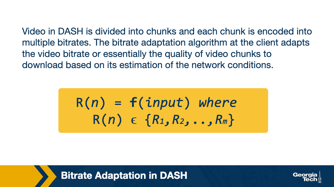
Here R(n) denotes the set of available bitrates.

The bitrate adaptation algorithm at the client adapts the video bitrate or essentially the quality of video chunks to download based on its estimation of the network conditions.

As you can imagine there can be different functions for bitrate adaptation that take into account different kinds of input. In the following topics, we will see different variations of how the bitrate adaptation function, f. We will talk about what kind of input it takes? How does it use the input to decide the quality of the video chunk? What does it try to optimize while doing bitrate adaptation, etc?

What are the Goals of Bitrate Adaptation?

Let us first look at what is the goal of the bitrate adaptation algorithm. A bitrate adaptation algorithm essentially tries to optimize the user's viewing quality of experience. A good quality of experience (QoE) is usually characterized by the following:

1. Low or zero re-buffering: users typically tend to close the video session if the video stalls a lot
2. High video quality: Better the video quality, better the user QoE. A higher video quality is usually characterized by high bitrate video chunk.
3. Low video quality variations: A lot of video quality variations are also known to reduce the user QoE.
4. Low startup latency: Startup latency is the time it takes to start playing the video since the user first requested to play the video. Players typically fill up the video buffer a little before playing the video. For this lesson, we will skip considering startup latency and focus on the other three metrics.

It is interesting to note that the different metrics characterizing QoE are conflicting. For instance, in order to have a high video quality, the player can download the higher bitrate chunks. However, it can lead to re-buffering if the network conditions are not good. Similarly, to avoid re-buffering, player can change either download the lowest bitrate, which leads to a low video quality, or change the video bitrate as soon as it notices a change in the network conditions, which leads to high video quality variations.

The goal of a good bitrate adaptation algorithm then is to consider these trade-offs and maximize the overall user Quality of experience.

Bitrate Adaptation Algorithms

Let us now look at what are the different signals that can serve as an input to a bitrate adaptation algorithm:

• Network Throughput: The first signal that can facilitate the selection of bitrate is the network conditions or more specifically the network throughput. Ideally, you would want to select a bitrate that is equal or lesser than the available throughput. Bitrate adaptation using this signal are known as rate-based adaptation.
• Video Buffer: The amount of video in the buffer can also enable to decide the video bitrate of the next chunk. For instance, if the video buffer is full, then the player can possibly afford to download high-quality chunks. Similarly, if the video buffer is low, the player can download low-quality chunks so as to quickly fill-up the buffer and avoid any re-buffering. Bitrate adaptation based on the video buffer is known as buffer-based adaptation.

In the remaining lesson, we will look at an example of each kind of adaptation algorithm. Note that in practice, players do end up using both the network throughput and the video buffer together for bitrate adaption.

Throughput-Based Adaptation and its Limitations

Let us first look at how throughput-based adaptation works.

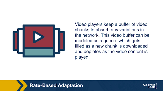
Recall that video players keep a buffer of video chunks to absorb any variations in the network. We can model this video buffer as a queue, which gets filled as a new chunk is downloaded and depletes as the video content is played.

Now, let us see what are the buffer filling and depletion rates?

The buffer-filling rate is essentially the network bandwidth divided by the chunk bitrate. For example, assume the available bandwidth is 10 Mbps, and the bitrate of the chunk is 1 Mbps. Then, in 1 second we can download 10s of video. Thus the buffer-filling rate is 10.

Now, the buffer-depletion rate or the output rate is simply 1. This is because 1s of video content gets played in 1s.

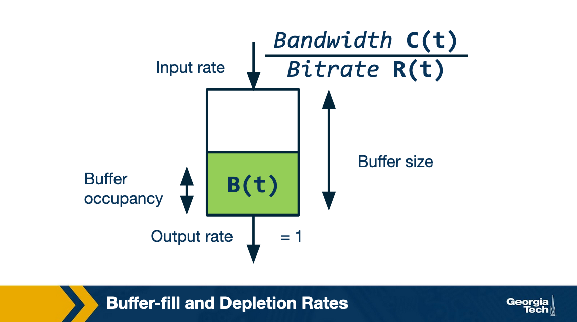
In order to have a stall-free streaming, clearly the buffer-filling rate should be greater than the buffer-depletion rate. In other words, C(t)/R(t) > 1 or C(t) > R(t).

However, C(t) is the future bandwidth and there is no way of knowing it. A good estimate of the future bandwidth is the bandwidth observed in the past. Therefore it uses the previous chunk throughput to decide the bitrate of the next chunk.

Rate-based Adaptation Mechanisms

A simple rate-based adaptation algorithm has the following steps:

1. Estimation: The first step involves estimating the future bandwidth. This is done by considering the throughput of the last few downloaded chunks. Typically, a smoothing filter such as moving average, or the harmonic mean is used over these throughputs to estimate the future bandwidth.
2. Quantization: In this the continuous throughput is mapped to discrete bitrate. Basically, we select the maximum bitrate that is less than the estimate of the throughput, including a factor in this selection.

Now, why do we add a factor? This is due of the following reasons:

1. We want to be a little conservative in our estimate of the future bandwidth to avoid any re-buffering
2. If the chunks are VBR-encoded, their bitrate can exceed the nominal bitrate
3. Finally, there are additional application and transport-layer overheads associated with downloading the chunk and we want to take them into account

Once the chunk-bitrate is decided, player sends the HTTP GET request for the next chunk. Note that a new chunk is not downloaded if the video buffer is already full. Instead, the player waits for the buffer to deplete before sending the next request. Once the new chunk is downloaded, its download throughput is also taken into account in estimating the next chunk's bitrate and the same process is repeated for downloading the next chunk.

Issues with Bitrate Adaptation

Now, we will look at an important issue in the above rate-based mechanism i.e. the issue of errors in future bandwidth estimation. Turns out in certain cases, rate-based adaptation ends up either overestimating or underestimating the future bandwidth which can lead to selection of a non optimal chunk bitrate. Let us look at each of the cases in detail.

Problem of Bandwidth OVER-Estimation with Rate-Based Adaption

Let us first look at how rate-based adaptation can lead to overestimation of bandwidth. Consider a case when the player is subjected to the following bandwidth where the bandwidth is 5 Mbps for the first 20 seconds and is then reduced to 375 kbps.

Let us assume the available bitrates are {250kbps, 500 kbps, 1 Mbps, 2 Mbps, 3 Mbps} and the chunk size is 3 Mbps. Initially, the player will stream at 3 Mbps. However, at t=20s the bandwidth goes down to 375 kbps which is high enough to play at the lowest bitrate. Assume the buffer occupancy at this time was 15s.

The video player has no way of knowing that the bandwidth has reduced. Therefore it ends up requesting a 3 Mbps chunk. To download this chunk, it will take 3 1000 5 / 375 seconds or 40 seconds. Meanwhile the video player buffer will deplete and the video will eventually re-buffer. If the player uses weighted average then it may even take more time to reflect the drop in the network bandwidth and the player may end up requesting higher bitrate than it should.

Thus, we can see under the case when the bandwidth changes rapidly, the player takes some time to converge to the right estimate of the bandwidth. As observed in this specific, this can sometimes lead to overestimation of the future bandwidth.

Problem of Bandwidth UNDER-Estimation with Rate-Based Adaption

Let us now look at a more interesting case of underestimation of the bandwidth.

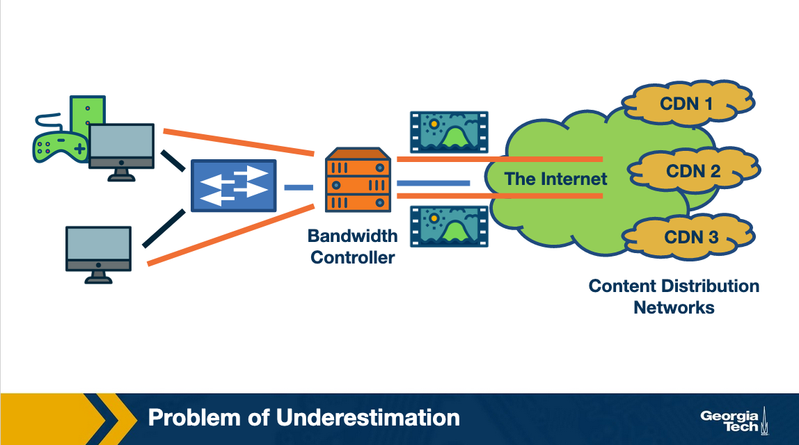
Consider the scenario when a client is watching a video over a 5Mbps link.

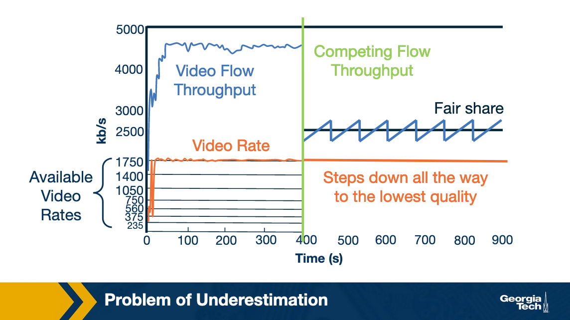
The available bitrates are {375kbps, 560 kbps, 750kbps, 1050kbps, 1400kbps, 1750kbs}. Clearly, the client would end up streaming at 1.75 Mbps under rate-based adaptation.

After some time another client joins in and starts downloading a large file. What would happen? Ideally, we would expect both clients to end up getting equal network bandwidth i.e. 2.5 Mbps as they are both using TCP. This means that the video client should continue streaming at 1.75 Mbps. However, the client ends up picking a lower bitrate and eventually goes down all the way to 235 kbps.

Let us see why this happens?

Recall that DASH clients have an ON-OFF pattern in the steady state. This happens when the video client has the buffer filled up and it is waiting for to deplete before requesting the next chunk.

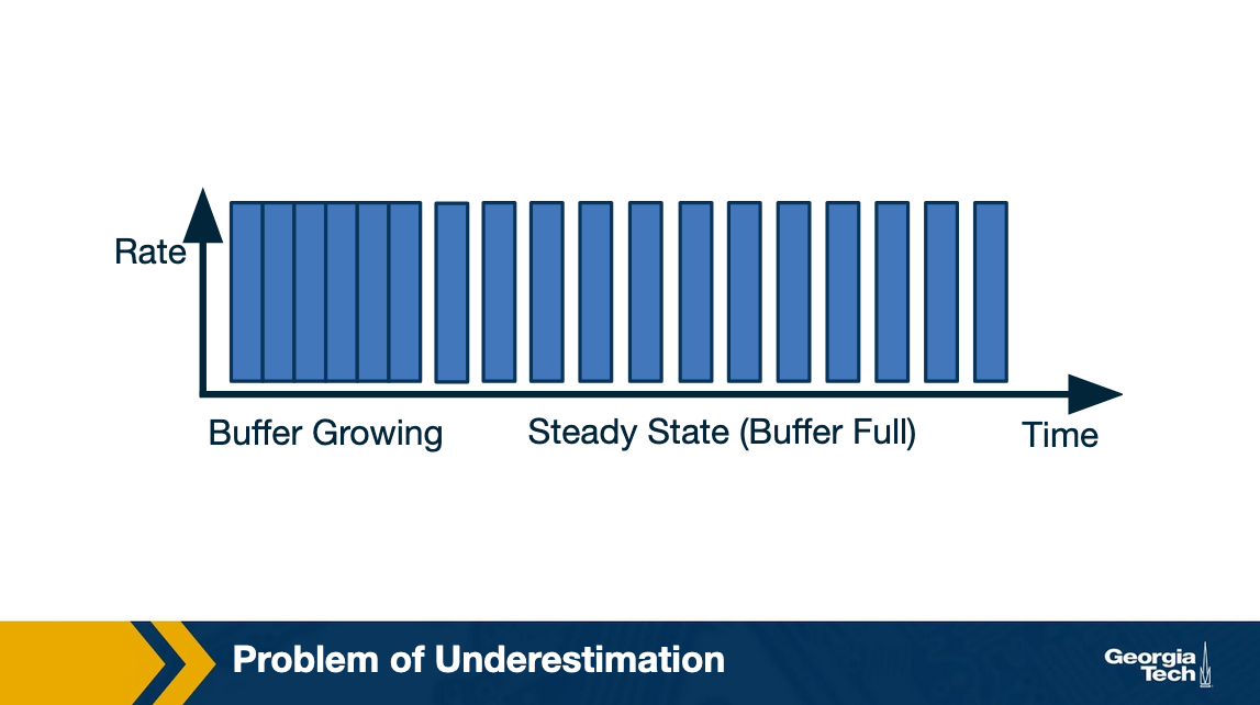
What can happen is that in this OFF period, the TCP connection reset the congestion window. Now this can impact the throughput observed for the chunk download as the TCP flow has another competing flow.

Recall that while TCP is fair, it does take time for the flows to converge to their fair share of the bandwidth. In our example, the chunk download can finish before TCP actually converges to the fair share.

In this example, say the observed throughput for the chunk was only 1.6 Mbps. Thus, it ends up picking a lower bitrate, i.e. 1050 kbps because of the rate-estimation being conservative (recall that players use a factor of alpha). Now, would it stabilize at that bitrate? Well, it turns out NO.

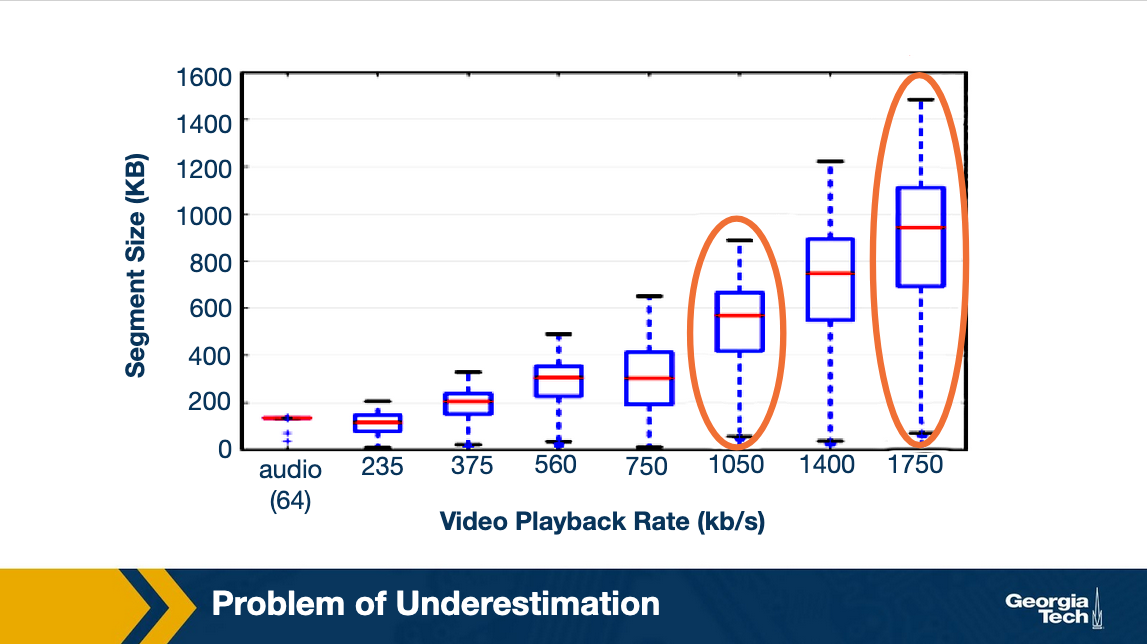
Here is a figure showing the size of chunks for different bitrates. As you can see, as the bitrate becomes lower, the chunk size reduces. This further aggravates the problem. In the presence of a competing flow, a smaller chunk size would lower the probability for the video flow to get its fair share. Thus, the player ends up further underestimating the network bandwidth and picks up even a lower bitrate until it converges to 235 kbps.

Note that this problem happens because of the ON-OFF behavior in DASH. Had it been two competing TCP-flows they would have gotten their fair share. While we have seen this problem for DASH and a competing TCP flow, it can also happen in competing DASH players leading to an unfair-allocation of network bandwidth.

Rate-Based Adaptation Conclusion

To summarize, rate-based adaptation pick the chunk bitrate based on estimation of available network bandwidth. While the actual available bandwidth is unknown and variable, it uses the past throughput as a proxy for the available bandwidth. This reactive estimation can lead the player to sometimes underestimate or overestimate the bandwidth under different scenarios.

Bitrate Adaptation Algorithm: Buffer-Based

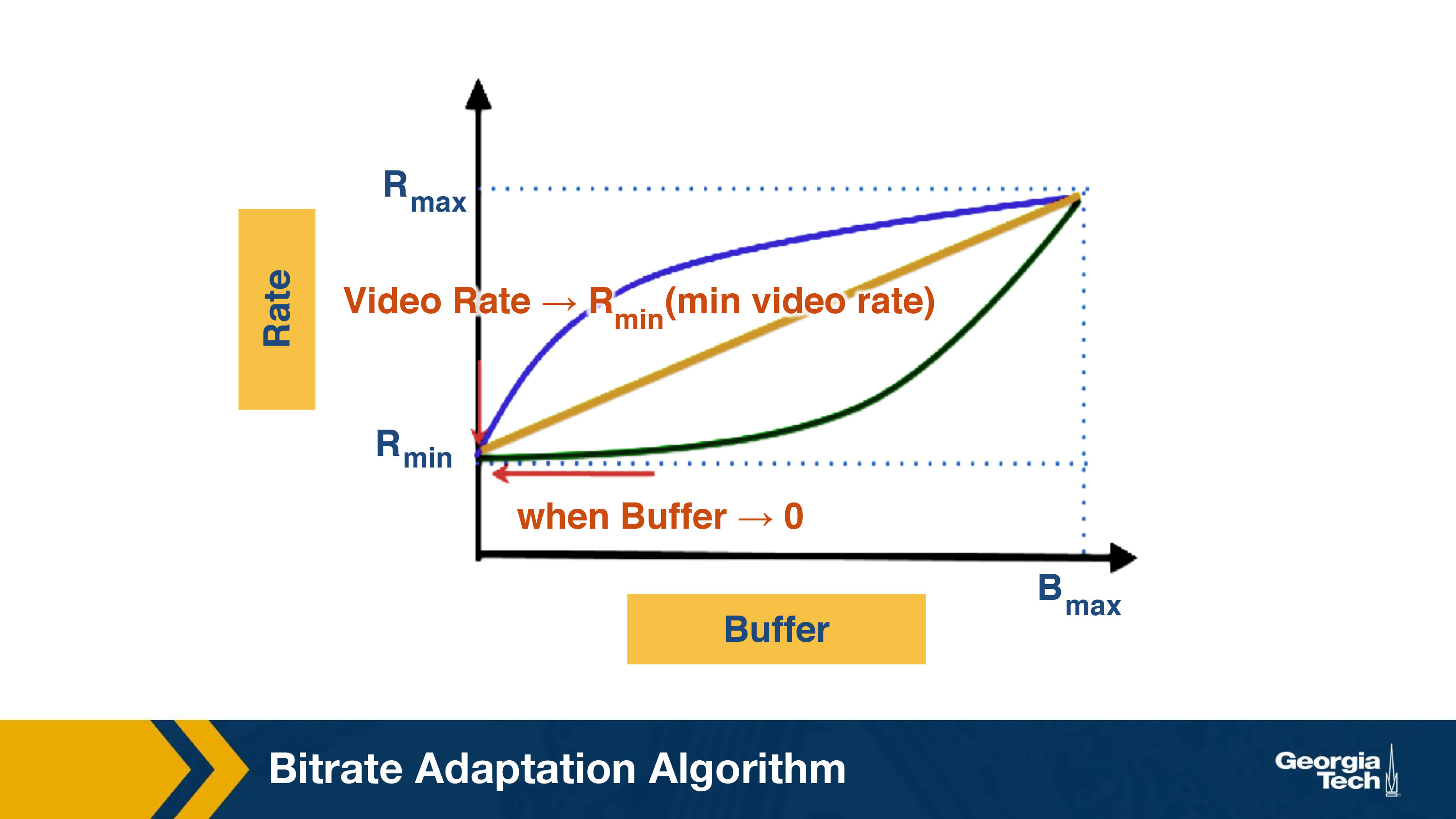
A second alternative is to use the buffer occupancy to inform bitrate selection. In other words, the bitrate of the chunk is a function of the buffer occupancy

R_next = f(buffer_now)

Now how should the function look like. The idea is quite simple: If the buffer occupancy is low, the player should download a low bitrate chunk and increase the chunk quality if the buffer occupancy increases. Thus, the bitrate adaptation function should be an increasing function with respect to the buffer occupancy. Figure below shows example functions, which are all increasing with respect to the buffer occupancy.

Using buffer-based adaptation can overcome the errors in bandwidth estimation that we saw in rate-based adaptation:

1. It avoids unnecessary re-buffering. As long as the download throughput is more than the minimum available bitrate, the video will not re-buffer. This is because, as the buffer occupancy becomes very low, it selects the minimum available bitrate.
2. It also fully utilizes the link capacity and does not suffer from bandwidth underestimation. This is because it avoids the on-off behavior as long as the video bitrate is less than the maximum available bitrate. Once the buffer occupancy is close to full, it starts requesting the maximum possible video bitrate.

Buffer-Based Adaptation Example

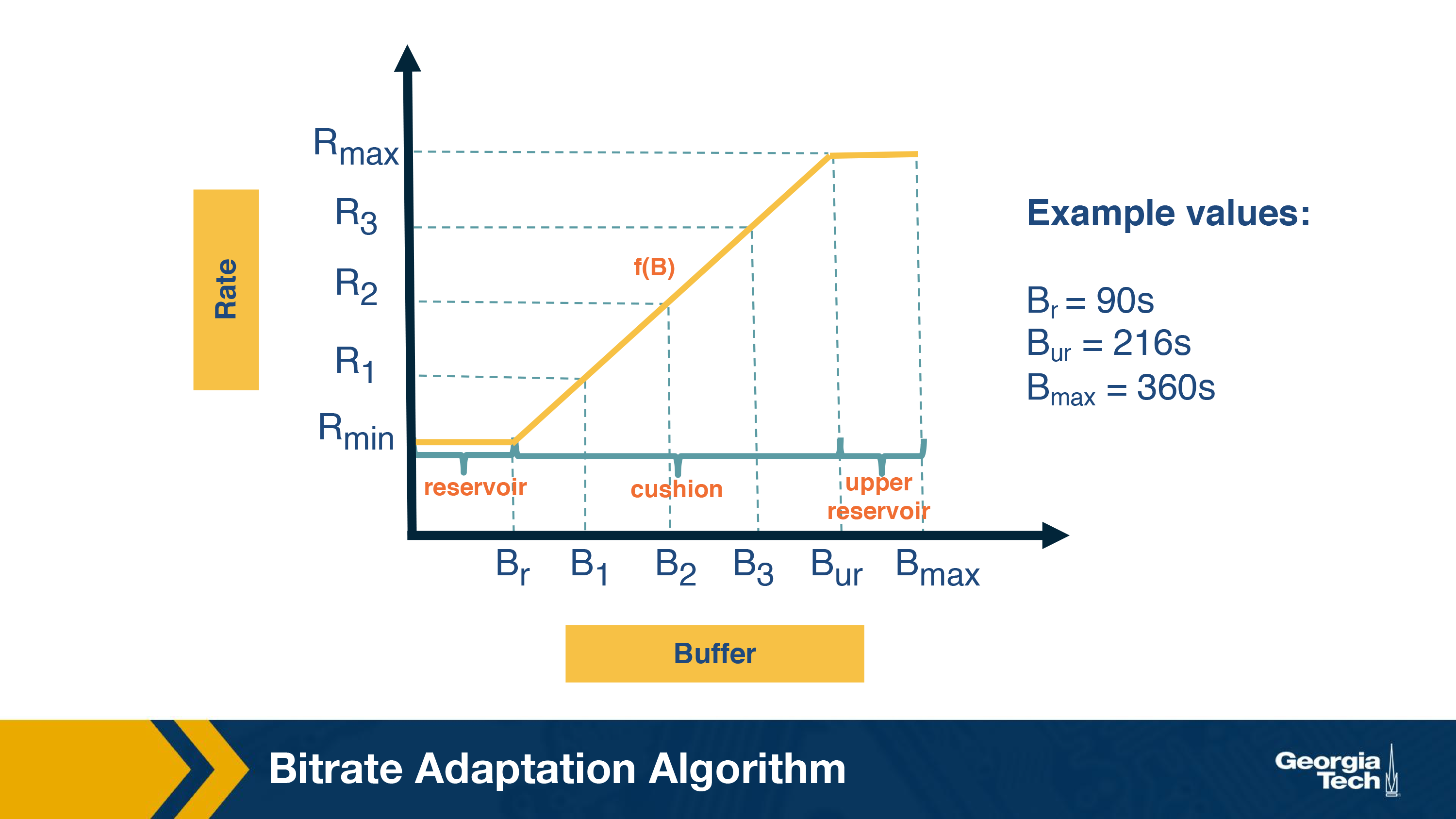
Here is an example buffer-based function. It has three regions of buffer occupancy. The reservoir region corresponds to low buffer occupancy and the player always selects the minimum available bitrate in this region. Similarly, when the buffer occupancy is in the upper reservoir region, the highest available bitrate is selected. Finally, in the middle or the cushion region, the bitrate is a linear function of the buffer occupancy. For instance, if the buffer is between B1 and B2, rate R1 is selected. The figure also shows example values for these regions.

Issues with Buffer-Based Adaptation

Even buffer-based adaptation has some issues.

1. In the startup phase, the buffer occupancy is zero. Therefore, the player will download a lot of low quality chunks which may be unnecessary.
2. It can lead to unnecessary bitrate oscillations. For instance, if the available bitrate is 1.5 Mbps and the available video bitrates are 1 Mbps and 2Mbps. The player will keep oscillating between these two. This is because if the player downloads 1 Mbps chunks, the buffer occupancy will increase and then it will start downloading 2 Mbps chunks. Since the available bandwidth is 1.5 Mbps, the buffer occupancy will decrease and then it will switch back again to 1Mbps.
3. Finally, it requires a large-buffer to implement the algorithm efficiently. This may not always be feasible. For instance, in the case of live streaming, the buffer size is not typically more than 8-16 seconds.

Bitrate Adaptation Conclusion

Thus, we saw two different flavors of bitrate adaptations and their associated advantages and disadvantages. Designing optimal bitrate adaptation algorithms is an active area of research. In practice, most video players use both the signals -- throughput and buffer occupancy -- together to decide the bitrate of the next chunk.

For instance, a recent paper from Sigcomm models bitrate adaptation as a QoE optimization problem:

https://www.cs.cmu.edu/~xia/resources/Documents/Yin_sigcomm15.pdf

A more recent paper models bitrate adaptation as a reinforcement learning problem:

https://people.csail.mit.edu/hongzi/content/publications/Pensieve-Sigcomm17.pdf