Intradomain Routing

Routing Algorithms

Let's assume that we have two hosts that have established a connection between them using TCP or UDP as we saw in the previous lecture.

Each of the two hosts know the default router (or first-hop router as we say). When a host sends a packet, the packet is first transferred to that default router. But what happens after that? In this lecture we will see the algorithms that we need so that when a packet leaves the default router of the sending host will travel over a path towards the default router of the destination host.

A packet will be able to travel from the sending host to the destination host with the help of intermediate routers. When a packet arrives at a router, the router is responsible to consult a forwarding table and then to determine the outgoing link interface to forward the packet. So by forwarding we refer to transferring a packet from an incoming link to an outgoing link within a single router. We will talk about forwarding in a following lecture.

By routing we refer to how routers work together using routing protocols to determine the good paths (or good routes as we call them) over which the packets travel from the source to the destination node.

When we have routers that belong to the same administrative domain we refer to the routing that takes place as intradomain routing.

But when the routers belong to different administrative domains, we refer to interdomain routing.

In this lecture we focus on intradomain routing algorithms or Interior Gateway Protocols (IGPs).

The two major classes of algorithms that we have are: A) link-state and B) distance-vector algorithms. For the following algorithms we represent each router as a node, and a link between two routers as an edge. Each edge is associated with a cost.

In this lecture, we discuss intradomain routing, where all the nodes and subnets are owned and managed by the same organization. (In contrast, interdomain routing is about routing between different organizations – such as between two ISPs.) Before we begin talking about intradomain routing algorithms, what could weights on the graph edges represent in these diagrams, when we are seeking the least-cost path between two nodes?

• Length of the cable
• Time delay to traverse the link
• Monetary cost
• Link capacity
• Current load on the link

Linkstate Routing Algorithm

In this topic, we will talk about the link state routing protocols, and more specifically about the Dijkstra's algorithm.

In the linkstate routing protocol, the link costs and the network topology are known to all nodes (for example by broadcasting these values).

Let's introduce some basic terminology. By u we represent our source node. By v we present every other node in the network. By D(v) we represent the cost of the current least cost path from u to v. By p(v) we present the previous node along the current least cost path from u to v. By N' we represent the subset of nodes along the current least-cost path from u to v.

Initialization step. We note that the algorithm starts with an initialization step, where we initialize all the currently known least-cost paths from u to its directly attached neighbors. We know these costs because they are the costs of the immediate links. For nodes in the network that they are not directly attached to u, we initialize the cost path as infinity. We also initialize the set N' to include only the source node u.

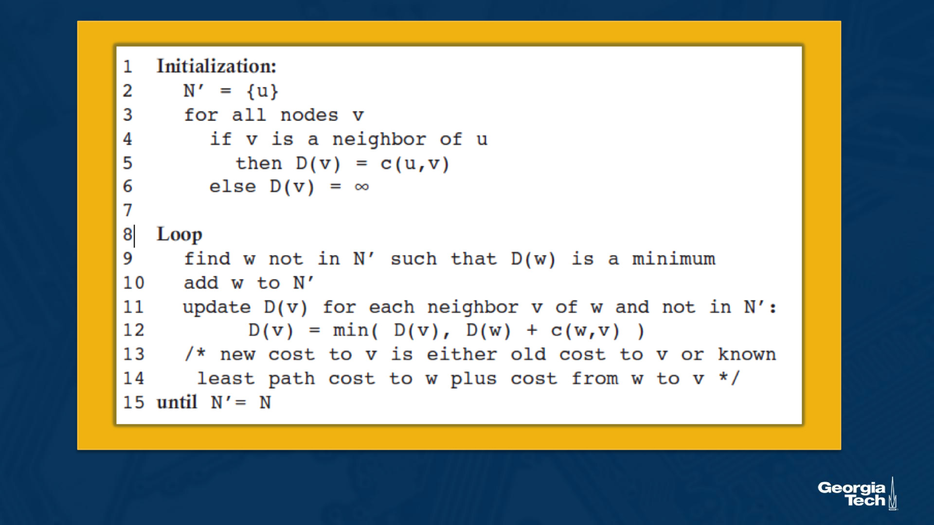
Iterations. After the initialization step, the algorithm follows with a loop that is executed for every destination node v in the network. At each iteration, we look at the set of nodes that are not included in N', and we identify the node (say w) with the least cost path from the previous iteration. We add that node w into N'. For every neighbor v of w, we update D(v) with the new cost which is either the old cost from u to v (from the previous iteration) or the known least path cost from source node u to w, plus the cost from w to v, whichever between the two quantities is the minimum.

The algorithm exits by returning the shortest paths, and their costs, from the source node u to every other node v in the network.

Linkstate Routing Algorithm - Example

Let's look at an example of the linkstate routing algorithm. We have the graph below and we consider our source node to be u. Our goal is to compute the least-cost paths from u to all nodes v in the network.

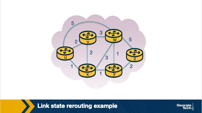
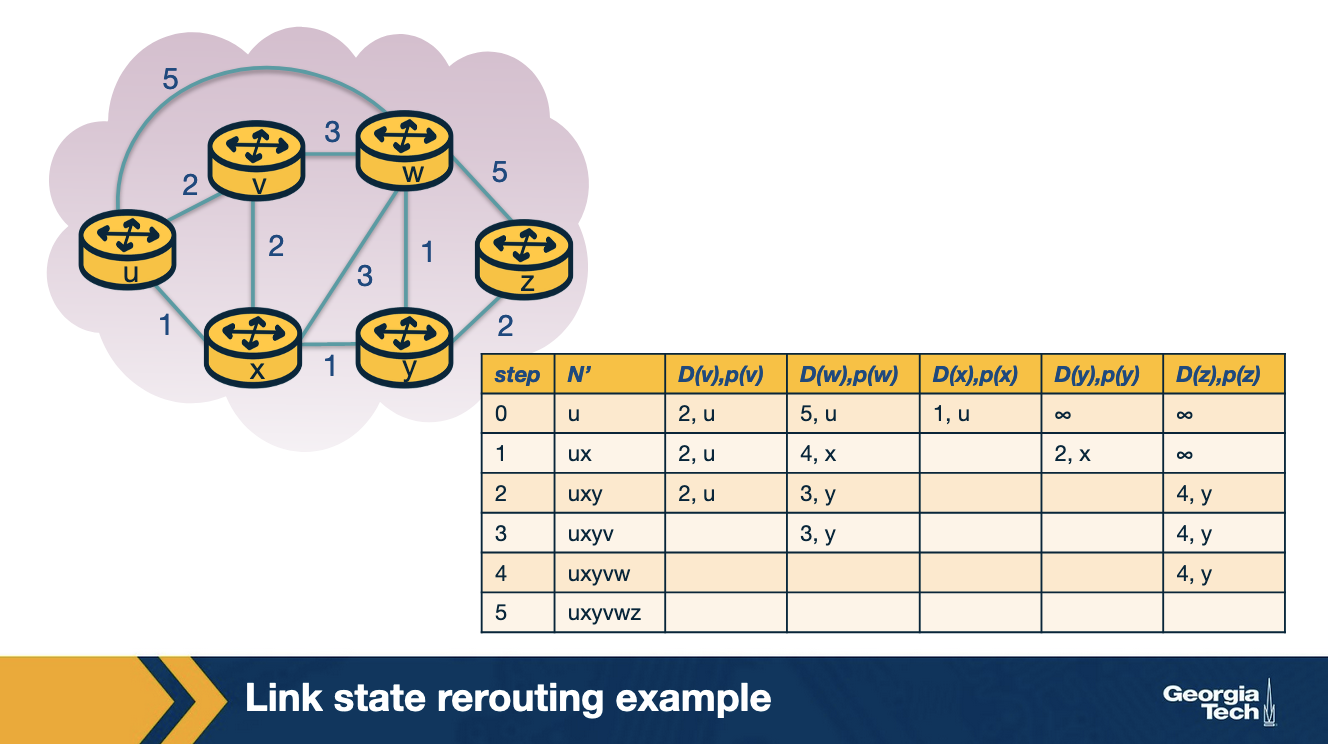
We start with the initialization step, where we set all the currently known least-cost paths from u to it's directly attached neighbors v, x and w. For the rest of the nodes in the network we set the cost to infinity, because they are not immediate neighbors to source node u. We also initialize the set N' to include only the source node u. The first row in our table represents the initialization step.

In the first iteration, we look among the nodes that are not yet in N', and we select the node with the least cost from the previous iteration. In this case, this is node x. Then we update D for all the immediate neighbors of x, which in this case are nodes v and w. For example, we update D(w) as the minimum between: the cost we had from the previous iteration which is 5, and the cost from u to x (1) plus cost from x to w (3). The minimum between the two is 4. We update the second row in our table.

We continue in a similar manner for the rest of the nodes in the table. The algorithm exits in the 5th iteration.

Linkstate Routing Algorithm - Computational Complexity

What is the computational complexity of the linkstate routing algorithm?

In other words, in the worst case, how many computations are needed to find the least-cost paths from the source to all destinations in the network? In the first iteration we need to search through all nodes to find the node with the minimum path cost. But as we proceed in the next iterations, this number decreases. So in the second iteration we search through (n-1) nodes. This decrease continues at every step. So by the end of the algorithm, after we go through all the iterations, we will need to search through n(n+1)/2 nodes. Thus the complexity of the algorithm is in the order of n squared O(n^2).

In the previous example, node u was the source node, and distances were calculated from u to each other node. Consider the same example, but let x be the source node. Notice that node x has more direct neighbors than u does. Suppose x is executing the linkstate algorithm as discussed, and has just finished the initialization step. Which of the following statements are true?

Node x will execute the same number of iterations that node u did, as the number of immediate neighbors has no impact on the number of iterations the algorithm requires.

Note that the algorithm continues iterating until

N' = N - 1

that is, until every node is the graph is in N'. As there are 6 nodes, there will always be 5 iterations after initialization.

Distance Vector Routing

In this section, we will talk about the distance vector routing algorithm.

The DV routing algorithm is iterative (the algorithm iterates until the neighbors do not have new updates to send to each other), asynchronous (the algorithm does not require the nodes to be synchronized with each other), and distributed (direct nodes send information to one another, and then they resend their results back after performing their own calculations, so the calculations are not happening in a centralized manner).

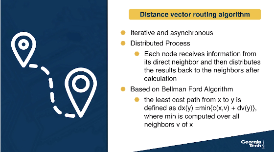
The DV algorithm is based on the Bellman Ford Algorithm. Each node maintains its own distance vector, with the costs to reach every other node in the network. Then, from time to time, each node sends its own distance vector to its neighbor nodes. The neighbor nodes in turn, receive that distance vector and they use it to update their own distance vectors. In other words, the neighboring nodes exchange their distance vectors to update their own view of the network.

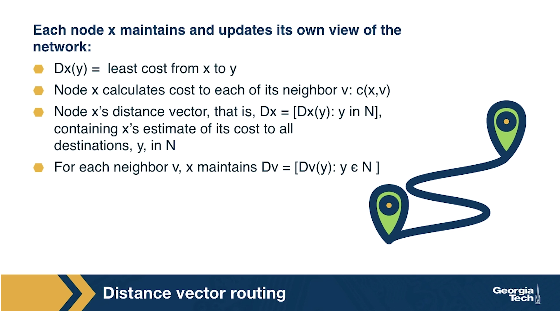
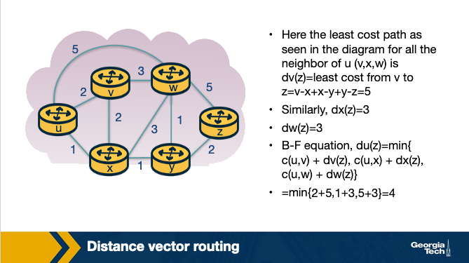
How the vector update is happening? Each node x updates its own distance vector using the Bellman Ford equation: Dx(y) = minv{c(x,v) + Dv(y)} for each destination node y in the network. A node x, computes the least cost to reach destination node y, by considering the options that it has to reach y through each of its neighbor v. So node x considers the cost to reach neighbor v, and then it adds the least cost from that neighbor v to the final destination y. It calculates that quantity over all neighbors v and it takes the minimum.

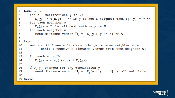
Formally, the DV algorithm is as follows:

Distance Vector Routing Example

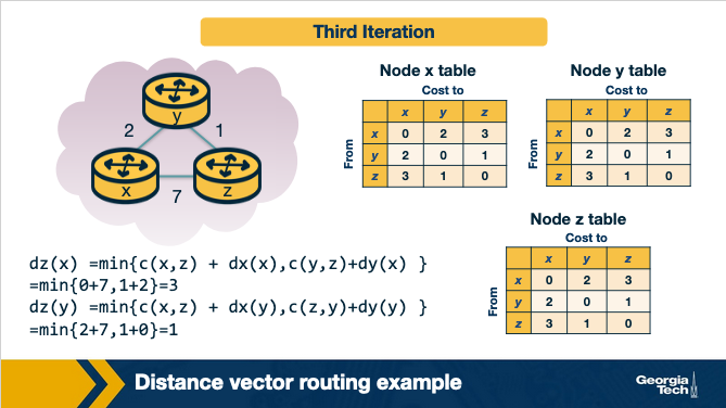
Now, let's see an example of the distance vector routing algorithm. Let's consider the three node network shown here:

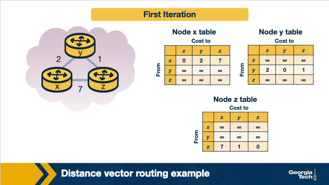
In the first iteration, each node has its own view of the network, which is represented by an individual table. Every row in the table is the distance vector of each node. Node x has it's own table, and the same is true for nodes y and z. We note that in the first iteration, node x does not have any information about the y's and z's distance vectors, thus these values are set to infinity.

In the second iteration, the nodes exchange their distance vectors and they update their individual views of the network.

Node x computes its new distance vector, using the Bellman Ford equation for every destination node y and z. For each destination, node x compares the cost to reach that destination through a neighbor node.

dx(y) = min{c(x,y) + dy(y), c(x,z)+dz(y) } = min{2+0, 7+1} = 2

dx(z) = min{c(x,y) + dy(z), c(x,z)+dz(z) } = min{2+1, 7+0} = 3

At the same time, node x receives the distance vectors from y and z from the first iteration. So it updates its table to reflect its view of the network accordingly.

Nodes y and z repeat the same steps to update their own tables.

In the third iteration, the nodes get the distance vectors from the previous iteration (if they have changed), and they repeat the same calculations. Finally, each node has its own routing table.

Finally, at this point, there are no further updates send from the nodes, thus the nodes are not doing any further calculations on their distance vectors. The nodes enter a waiting mode, until there is a change in the link costs.

Link Cost Changes and Failures in DV - Count to Infinity Problem

Now, we will see what is happening when a node identifies that a link that it is connecting it to one of its neighbors as changed.

Let's consider the following example topology below:

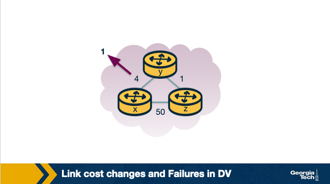
Let's assume that the link cost between x-y changes to 1.

1. At time t0, y detects that cost to x has changed from 4 to 1, so it updates its distance vector and sends it to its neighbors.
2. At time t1, z receives the update from y. Now it thinks that is can reach x through y with a cost of 2. And it sends its new distance vector to its neighbors.
3. At time t2, y receives update from z. Y distance vector does not change its distance vector and does not send updates.

In this scenario, we note that the fact that there was a decrease in the link cost, it propagated quickly among the nodes, as it only took a few iterations.

Unfortunately, this is not always the case. Let's consider the following scenario where a link cost increases by a large amount.

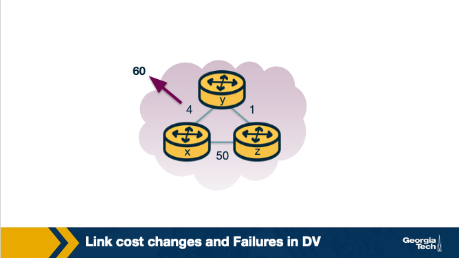
Let's assume that the link y-x has a new cost of 60.

1. At t0, y detects that cost has changed, now it will update its distance vector thinking that it can still reach x through z with a total cost of 5+1=6 (path cost z to x + path cost y to z since y thinks it can reach x faster this way)
2. At t1, we have a routing loop, where z thinks it can reach x through y and y thinks it can reach x through z. This will be causing the packets to be bouncing back and forth between y and z until their tables change.
3. z and y keep updating each other about their new cost to reach x. For example, y computes its new cost to be 6, it informs z. Then z computes its new cost to be 7, and it informs y, and so on.

This back and forth continues for a total of 44 iterations, at which point z computes its cost to be larger than 50, and that point it will prefer to reach x directly rather than through y.

In contrast to the previous scenario, this link cost change took a long time to propagate among the nodes of the network. This is known as the count-to-infinity problem.

Poison Reverse

A solution to the previous problem is the following idea, called poison reverse: since z reaches x through y, z will advertise to y that the distance to x is infinity (Dz(x)=infinity). However z knows that this is not true and Dz(x)=5. z tells this lie to y, as long as it knows that it can reach to x via y. Since y assumes that z has no path to x except via y, it will never send packets to x via z.

So z poisons the path from z to y.

Things change when the cost from x to y changes to 60. y will update its table and send packet to x directly with cost Dy(x)=60. It will inform z about its new cost to x, after this update is received. Then z will immediately shift its route to x to be via the direct (z,x) link at cost 50. Since there is a new path to x, z will inform y that Dz(x)=50.

When y receives this update from z, y will update Dy(x)=51=c(y,z)+Dz(x).

Since z is now on least cost path of y to reach x, y poisons the reverse path from z to x by. Y tells z that Dy(x)=inf, even though y knows that Dy(x)=51.

This technique will solve the problem with 2 nodes, however poisoned reverse will not solve a general count to infinity problem involving 3 or more nodes that are not directly connected.

Distance Vector Routing Protocol Example: RIP

The Routing Information Protocol (RIP) is based on the Distance Vector protocol.

The first version, released as a part of the BSD version of Unix, uses hop count as a metric (i.e. assumes link cost as 1). The metric for choosing a path could be shortest distance, lowest cost or a load-balanced path. In RIP, routing updates are exchanged between neighbors periodically, using a RIP response message, as opposed to distance vectors in the DV Protocols. These messages, called RIP advertisements, contain information about sender's distances to destination subnets.

Let's look at a simple RIP example to illustrate how it works. The figure below shows a portion of the network. Here, A, B, C and D denote the routers and w, x, y and z denote the subnet masks.

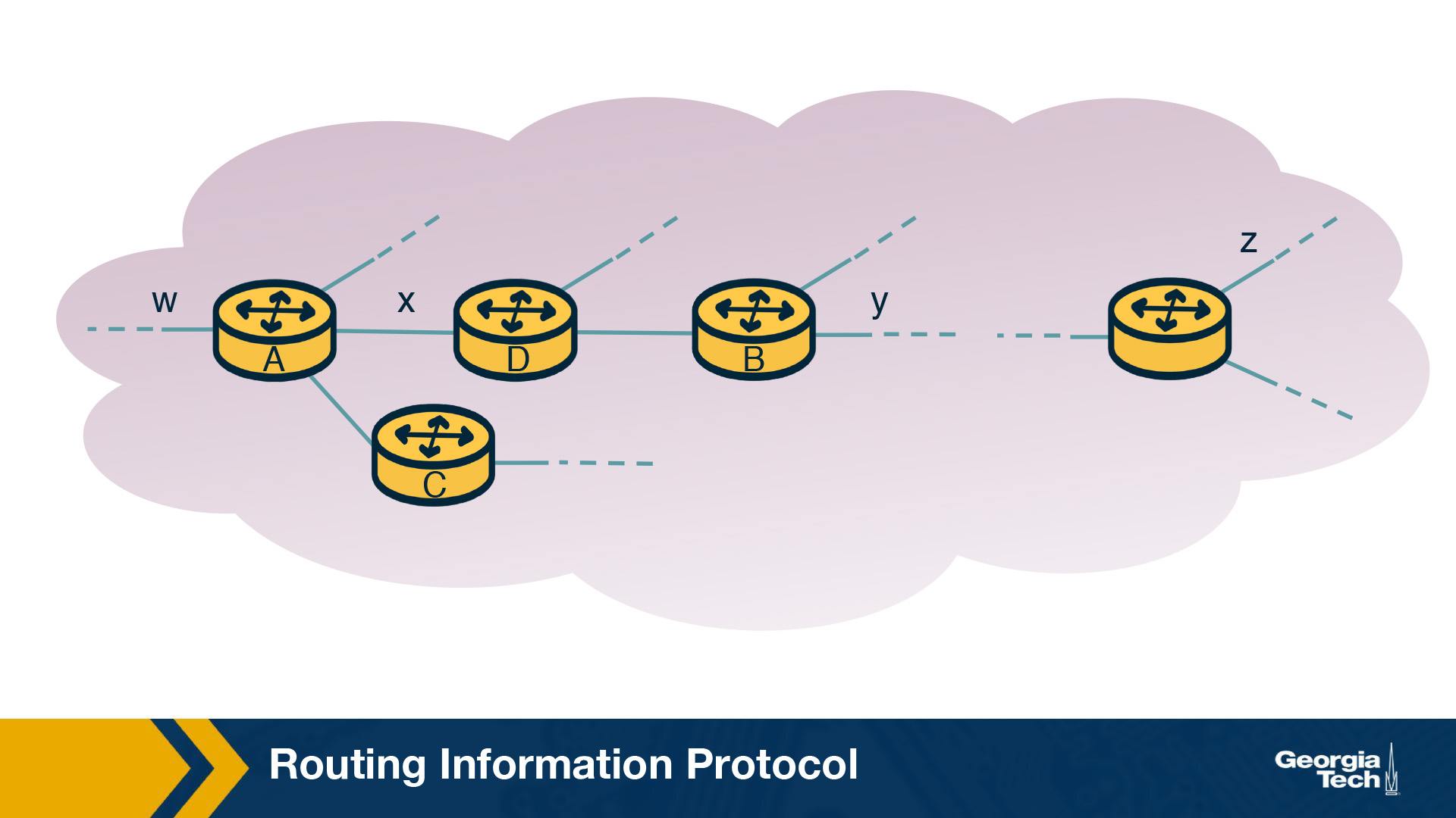
Each router maintains a routing table, which contains its own distance vector as well as the router's forwarding table. If we have a look at the routing table of Router D, we will see that it has three columns: destination subnet, identification of the next router along the shortest path to the destination, and the number of hops to get to the destination along the shortest path. A routing table will have one row for each subnet in the AS.

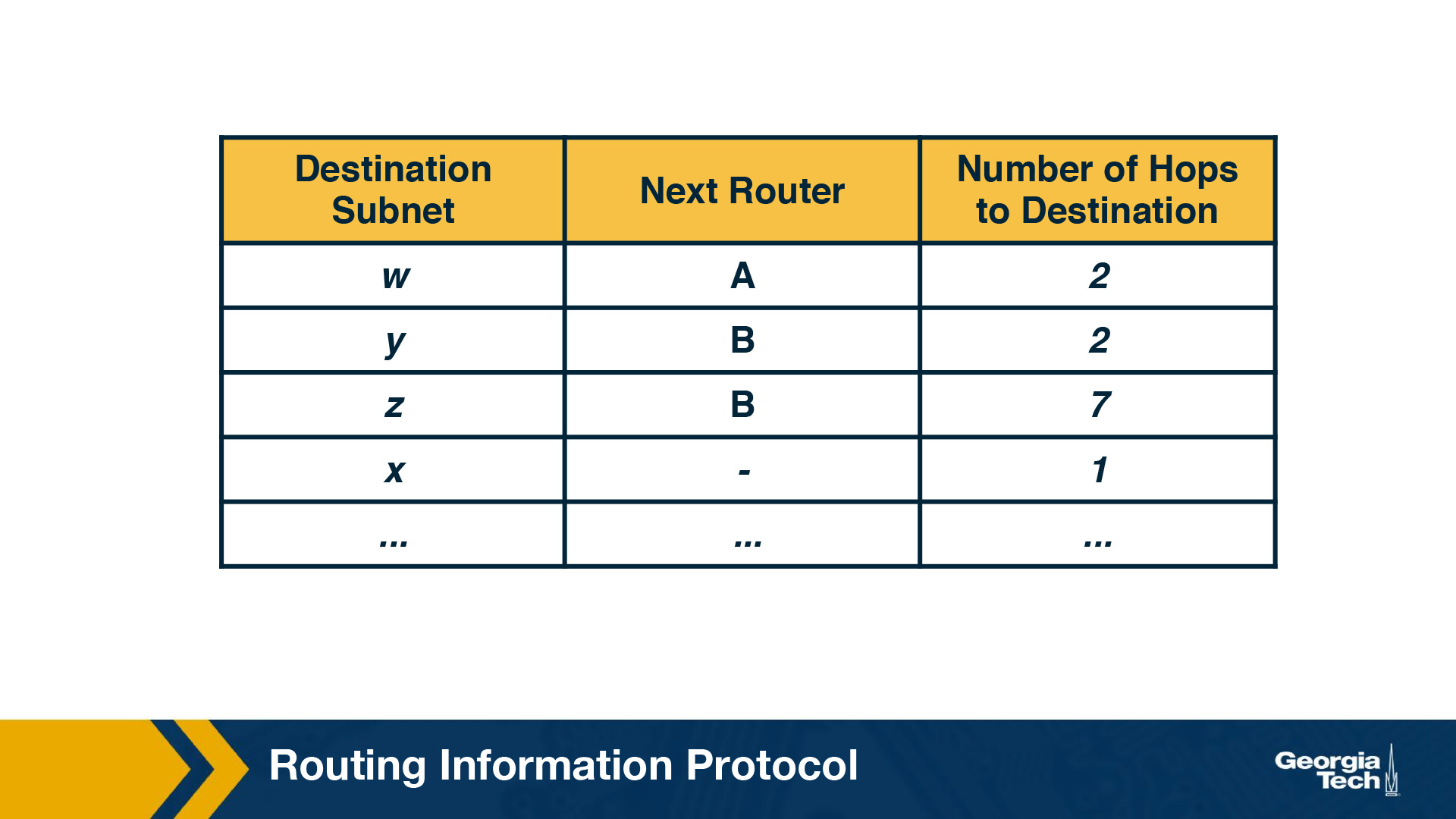
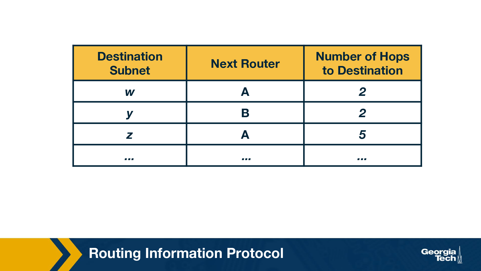
For this example, the table in the above figure indicates that to send a datagram from router D to destination subnet w, the datagram should first be forwarded to neighboring router A; the table also indicates that destination subnet w is two hops away along the shortest path. Now if router D receives from router A the advertisement (the routing table information of router A) shown in the figure below it merges the advertisement with the old routing table.

In particular, router D learns that there is now a path through router A to subnet z that is shorter than the path through router B. Therefore, router D updates its table to account for the new shortest path. The updated routing table is shown in the figure below. As the Distance Vector algorithm is in the process of converging or as new links or routers are getting added to the AS, the shortest path is changing.

Each node maintains a RIP Table (Routing Table), which will have one row for each subnet in the AS. RIP version 2 allows subnet entries to be aggregated using route aggregation techniques.

If a router does not hear from its neighbor at least once every 180 seconds, that neighbor is considered to be no longer reachable (broken link). In this case, the local routing table is modified and changes are propagated. Routers send request and response messages over UDP, using port number 520, which is layered on top of network-layer IP protocol. RIP is actually implemented as an application-level process.

Some of the challenges with RIP include updating routes, reducing convergence time, and avoiding loops/count-to-infinity problems.

Linkstate Routing Protocol Example: OSPF

Open Shortest Path First (OSPF) is a routing protocol which uses a link state routing algorithm to find the best path between the source and the destination router. OSPF was introduced as an advancement of the RIP Protocol, operating in upper-tier ISPs. It is a link-state protocol that uses flooding of link-state information and a Dijkstra least-cost path algorithm. Advances include authentication of messages exchanged between routers, the option to use multiple same cost paths, and support for hierarchy within a single routing domain.

As we have seen already, a link state routing algorithm is a dynamic routing algorithm in which each router shares knowledge of its neighbors with every other router in the network. The network topology that is built as a result can be viewed as a directed graph with preset weights for each edge assigned by the administrator.

Hierarchy. An OSPF autonomous system can be configured hierarchically into areas. Each area runs its own OSPF link-state routing algorithm, with each router in an area broadcasting its link state to all other routers in that area. Within each area, one or more area border routers are responsible for routing packets outside the area.

Exactly one OSPF area in the AS is configured to be the backbone area. The primary role of the backbone area is to route traffic between the other areas in the AS. The backbone always contains all area border routers in the AS and may contain non-border routers as well.

For packets routing between two different areas, it is required that the packet be sent through an area border router, through the backbone and then to the area border router within the destination area, before finally reaching the destination.

Operation. First, a graph (topological map) of the entire AS is constructed. Then, considering itself as the root node, each router computes the shortest-path tree to all subnets, by running Djikstra's algorithm locally. The link costs have been pre-configured by a network administrator. The administrator has a variety of choices while configuring the link costs. For instance, he may choose to set them to be inversely proportional to link capacity, or set them all to one. Given set of link weights, OSFP provides the mechanisms for determining least-cost path routing.

Whenever there is a change in a link's state, the router broadcasts routing information to all other routers in the AS, not just to its neighboring routers. It also broadcasts a link's state periodically even if its state hasn't changed.

Link State Advertisements. Every router within a domain that operates on OSPF uses Link State Advertisements (LSAs). LSA communicates the router's local routing topology to all other local routers in the same OSPF area. In practice, LSA is used for building a database (called the link state database) containing all the link states. LSAs are typically flooded to every router in the domain. This helps form a consistent network topology view. Any change in the topology requires corresponding changes in LSAs.

Refresh rate for LSAs. OSPF typically has a refresh rate for LSAs, which has a default period of 30 minutes. If a link comes alive before this refresh period is reached, they routers connected to that link ensure LSA flooding. Since the process of flooding can happen multiple times, every router receives multiple copies of refreshes or changes - and stores the first received LSA change as new, and the subsequent ones as duplicates.

Processing OSPF Messages in the Router

In the previous section, we looked at OSPF fundamentals and how it operates using Link State Advertisements (LSA). In this section we will look at how the OSPF messages are processed in the router in more detail.

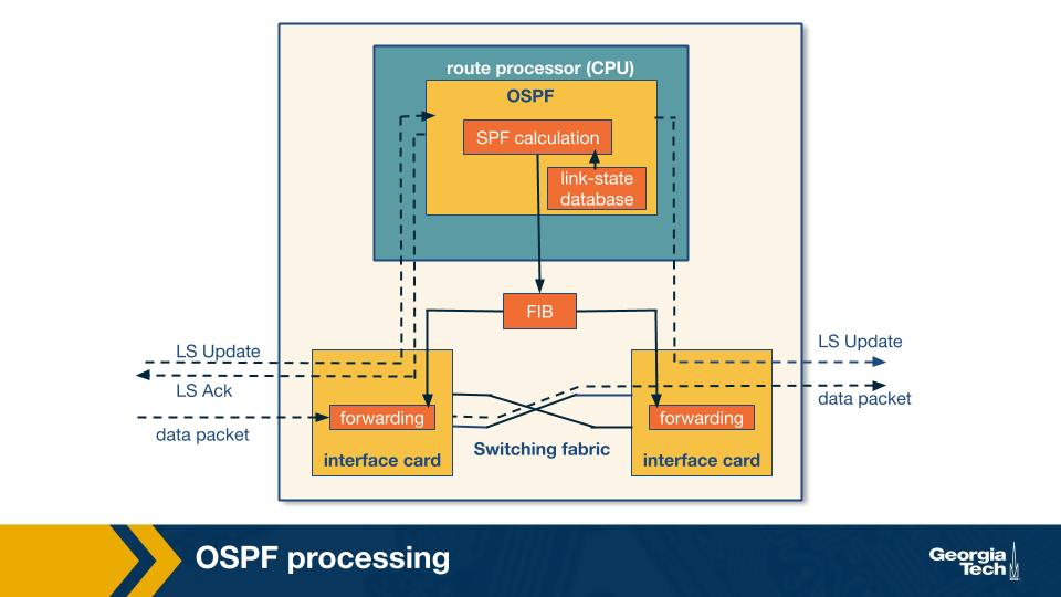
To do this, let's begin with a simple model of a router given in the figure above. The router consists of a route processor (which is the main processing unit) and interface cards that receive data packets which are forwarded via a switching fabric. Let us break down router processing in a few steps:

1. Initially, the LS update packets which contain LSAs from a neighboring router reaches the current router's OSPF (which is the route processor). This is the first trigger for the route processor. As the LS Updates reach the router, a consistent view of the topology is being formed and this information is stored in the link-state database. Entries of LSAs correspond to the topology which is actually visible from the current router.
2. Using this information from the link-state database, the current router calculates the shortest path using shortest path first (SPF) algorithm. The result of this step is fed to the Forwarding Information Base (FIB)
3. The information in the FIB is used when a data packet arrives at an interface card of the router, where the next hop for the packet is decided and its forwarded to the outgoing interface card.

To further understand OSPF processing, let's look at the following flow chart and view it in time slices (T1, T2, …, T7).

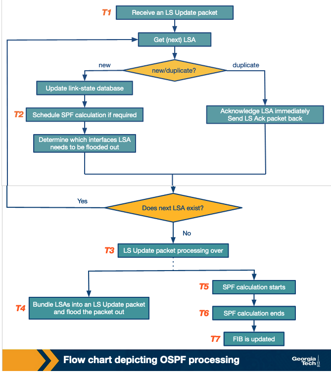
We've already noted that the processing tasks begin at the receipt of an LS update packet (T1). For every LSA unpacked from the update packet, the OSPF protocol checks whether it is a new or a duplicate LSA. This is done by referring to the link-state database, and checking for the sequence number of the LSA to a matching LSA instance in the database. For every new LSA, the database is updated, an SPF calculation is scheduled (T2) and it's determined which interface the LSA needs to be flooded out of. In modern routers, the when of LSA flooding can be based on a timer.

When all the LSAs from an LS update packet have been processed (T3), the LSAs are prepared and flooded out as an LS Update packet to the next router (T4). After this, we move on to the actual execution of SPF calculation within the router (T5 and T6). Since SPF calculation is a CPU-intensive task, SPF calculations are scheduled and carried out over a period of time (usually when LSA's are changed) so as to offset the CPU costs. After the SPF calculation is completed, the FIB is updated (T7).

Hot Potato Routing

In large networks, routers rely both on interdomain and intradomain routing protocols to route the traffic.

The routers within the network use the intradomain routing protocols to find the best path to route the traffic within the network. In case when the final destination of the traffic is outside the network, then the traffic will travel towards the networks exit (egress points) before leaving the network. In some cases there are multiple egress points that the routers can choose from. These egress points (routers) can be equally good in the sense that they offer similarly good external paths to the final destination.

In this case, hot potato routing is a technique/practice of choosing a path within the network, by choosing the closest egress point based on intradomain path cost (Interior Gateway Protocol/IGP cost).

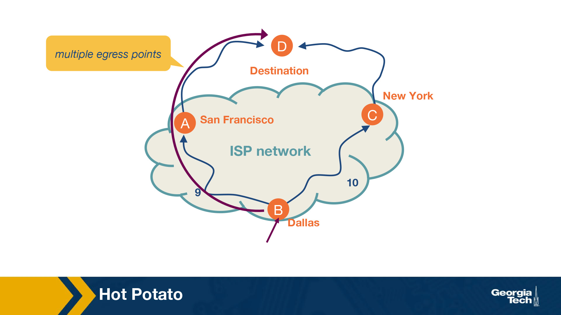
Let's look at an example.

In the figure above, we have a network, and specifically we are looking at the a router located in Dallas and the router needs to forward traffic towards a destination. It could do so via New York or San Francisco. We assume that both egress points offer BGP (Border Gateway Protocol) path costs, so they are equally good egress points. In this case, the router has multiple egress points. We see that the IGP path cost for SF is 9 while the path cost for NY is 10. Thus, the router uses hot potato routing to choose to send the traffic to the destination via SF.

Hot potato routing simplifies computations for the routers as they are already aware of the IGP path costs. It makes sure that the path remains consistent, since the next router in the path will also choose to send the packet to the same egress point.

Hot potato routing also effectively reduces the network's resource consumption by getting the traffic out as soon as possible.

Example Traffic Engineering Framework

In this section we will see an example traffic engineering framework. It involves three main components: measure, model and control as shown in the below figure.

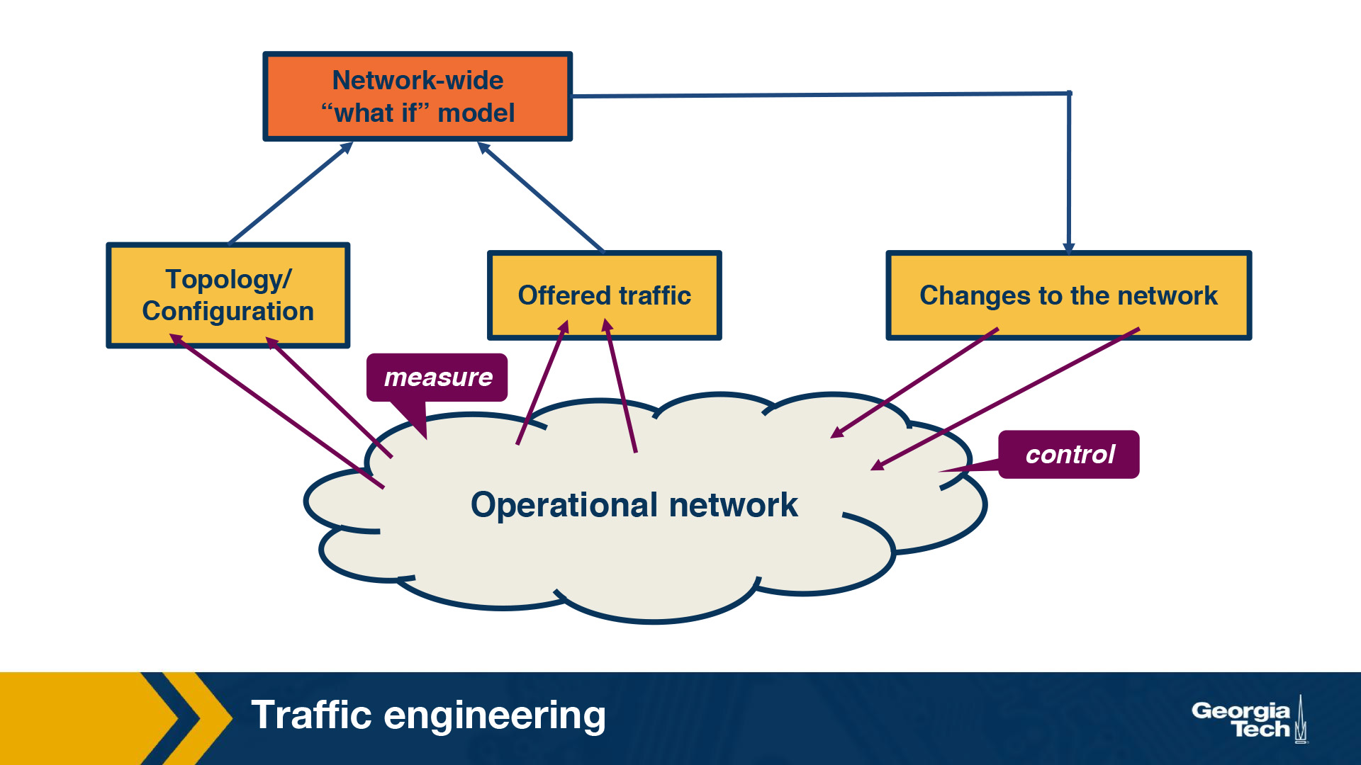
As a first step, the network operator measures the topology of the network and traffic demands. The next step involves predicting the effect of change in IGP parameters on the traffic flow to evaluate different link weights. Finally, once the weights are decided, the new values are updated on the routers.

Measure: The efficient assignment of link weights depends on the real time view of the network state which includes:

• the operational routers and links,
• the link capacity and IGP parameters configuration.

The status of the network elements can be obtained using Simple Network Management Protocol (SNMP) polling or via SNMP traps. The link capacity and the IGP parameters can be gathered from the configuration data of the routers or external databases that enable the provisioning of the network elements. Furthermore, a software router could act as an IGP route monitor by participating in OSPF/IS-IS with operational routers and reporting real time topology information.

In addition to the current network state, the network operator also requires an estimate of the traffic in the network that can be acquired either by prior history or by using the following measurement techniques:

1. Directly from the SNMP Management Information Bases (MIBs)
2. By combining packet-level measurements at the network edge using the information in routing tables
3. Network tomography which involves observing the aggregate load on the links along with the routing data
4. Direct observation of the traffic using new packet sampling techniques

Model: This involves predicting the traffic flow through the network based on the IGP configuration. The best path between two routers is selected by calculating the shortest path between them when all the links belong to the same OSPF/IS-IS area. In case of large networks consisting of multiple OSPF/IS-IS areas, the path selection among routers in different areas is dependent on the summary information passed across the area boundaries. If there are multiple shortest paths between two routers, it is leveraged for load balancing by splitting the traffic almost evenly over these paths.

The routing model thus aims to compute a set of paths between each pair of routers, with each path representing the fraction of traffic that passes through each link. The volume of traffic on a link can now be estimated by combining the output of the routing model and the estimated traffic demands.

Control: The new link weights are applied on the affected routers by connecting to the router using telnet or ssh. The exact commands are dependent on the operating systems of the router. These updates may be automated or done manually depending on the size of the network.

Once a router receives a weight change, it updates its link-state database and floods the newly updated value to the entire network. On receiving the updated value, each router in turn updates its link-state database, recomputes the shortest paths and updates affected entries in its forwarding table. Similar to when there is a topology change or a failure, this involves a transition period where there is a slightly inconsistent view of the shortest path for few destinations. Although the convergence after a weight change is faster than a failure scenario (as there is no delay in detecting a failure), it still involves a transient period in the network. Hence, understandably, changing the link weights is not done frequently and only done in scenarios where there is new hardware, equipment failures or changes in traffic demands.