Relational Algebra and Calculus

Closed Algebra

Let's talk about closed algebra. Consider the following expression containing rational numbers:

Even if we can't discern the result by looking at the expression, we know the steps required to compute the result based on the rules governing the order of operations.

We call this algebra closed because each expression involving rational numbers evaluates to a rational number, resolving to the same type of data as we input. A closed algebra allows you to formulate high-level models and use previous thoughts to form new ones. In the expression above, we build up intermediate results from the initial operands until we finally arrive at one value.

Relational Algebra Operations

Let's look at a collection of relational algebra operators involving two relations, $R$, and $S$. First, we have four set operators:

• The set union operator, $R \cup S$
• The set intersection operator, $R \cap S$
• The set difference operator, $R \setminus S$
• The Cartesian product operator, $R \times S$

We use the projection operator, $\pi$, to eliminate attributes, or columns, from a relation. For example, $\pi_{A_1, A_2, ..., A_n}(R)$ selects only those attributes $A_1, A_2, ... , A_n$ in $R$. We use the selection operator $\sigma$, which eliminates rows. For example, $\sigma_{\text{expression}}(R)$ selects only those rows in $R$ for which $\text{expression}$ evaluates to true.

The third group of operators is the joins, which are constructor operations. We have the natural join operator, $R * S$. We also have outer joins, of which there are three types: right, left, and full. In this lesson, we look at left outer joins, $\Join_{\text{L}}$. Finally, we have theta joins, $R \Join_\theta S$.

In the last group of operators, we see the division operator, $R \div S$, and the rename operator, $\rho$. Division in relational algebra provides functionality similar to universal quantification in relational calculus. The rename operator lets us rename relation attribute names so two relations can have the same name for certain attributes and thus be joined on them.

The symbol for the left outer join is not really $\Join_{\text{L}}$. It's the symbol shown in the lectures. Unfortunately, it's not in my character set in this environment, so I can't express it.

Selection

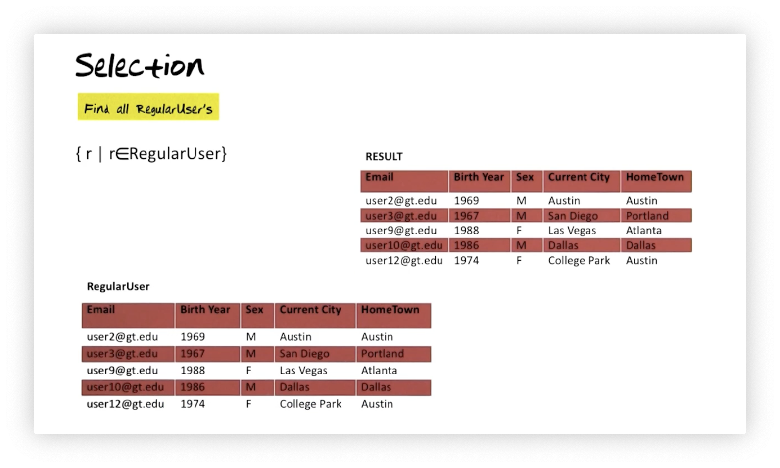
The general syntax to select all the tuples from a relation, $R$, that satisfy an expression is $\sigma_\text{expression}(R)$. For example, if we want to retrieve all tuples in the RegularUser relation, we would say:

If RegularUser has $n$ tuples, the resulting relation after running this query will also have $n$ tuples in it because we haven't specified any condition to eliminate tuples.

Selection - Simple Expression

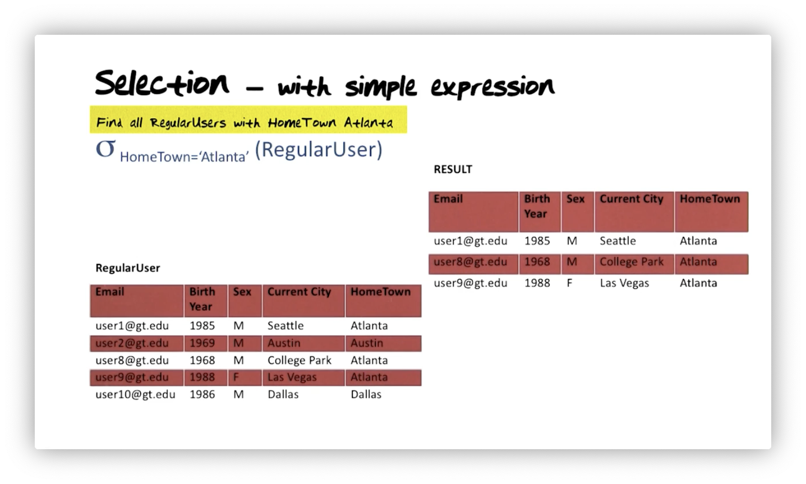
Let's look at the selection operator with a simple expression. Suppose we want to find all regular users whose hometown is Atlanta. We can express that query in relational algebra as:

We can form simple expressions in one of two ways: either we can compare two attributes or an attribute to a constant. The comparison operators we have at hand are $=$, $<$, $\leq$, $>$, $\geq$, and $\neq$.

In the RegularUser table, we now select all tuples with a value of 'Atlanta' for the HomeTown attribute. Remember, when we perform a selection, we retain the number of columns from the original relation in the selection result.

Selection - Composite Expression

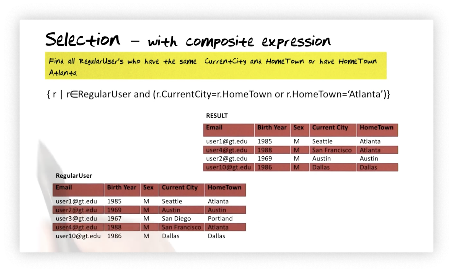
Suppose we want to find all regular users with the same current city and hometown or with a hometown of Atlanta. We can express this query as so:

Notice that the result of this selection, shown below, includes users who have a hometown in Atlanta and those whose hometown matches their current city. For example, we see one user from Dallas who currently lives in Dallas and another user from Austin who currently lives in Austin.

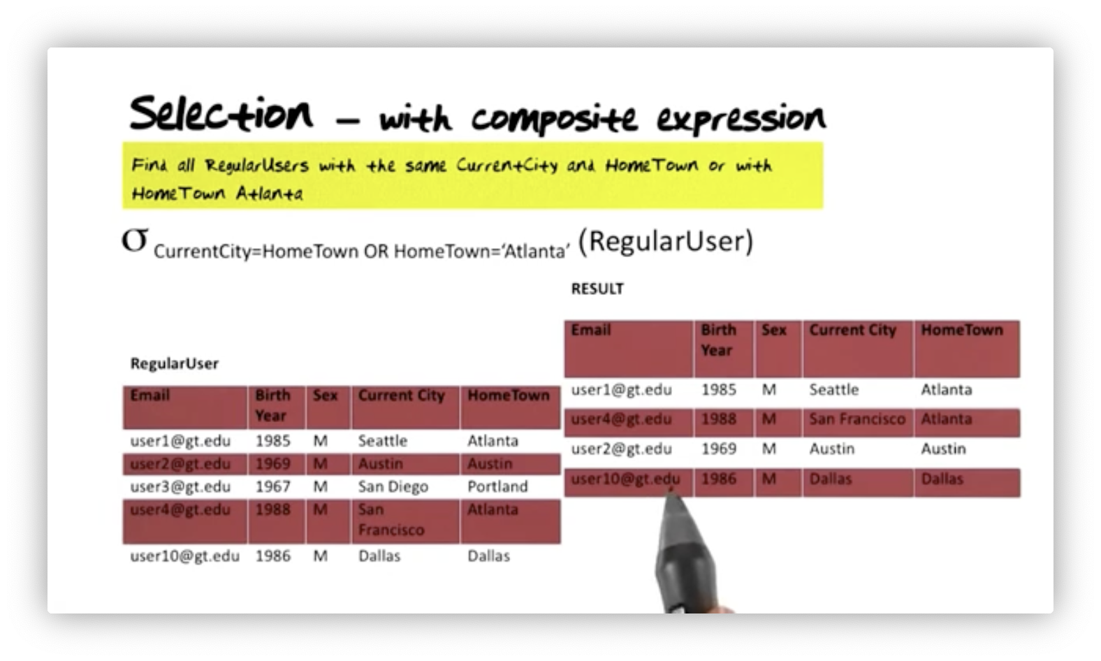
We can form composite expressions by combining simple expressions. Conjunction, expressed mathematically as $\land$, refers to 'AND'ing two expressions, disjunction, $\lor$, refers to 'OR'ing them, and negation refers to inverting the truthiness of an expression. Additionally, we can place parenthesis around an expression, which gives us fine control over the order of operations.

Projection

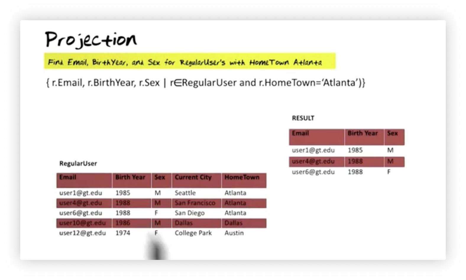
Given a relation, $R$, and attributes, $A = \{ A_1, A_2,...,A_n \}$, where $A$ forms a subset of the attributes on $R$, we can project $A$ from $R$ like so:

For example, suppose we want to retrieve just the email, birth year, and sex for all regular users in Atlanta. We can express this query with the following syntax:

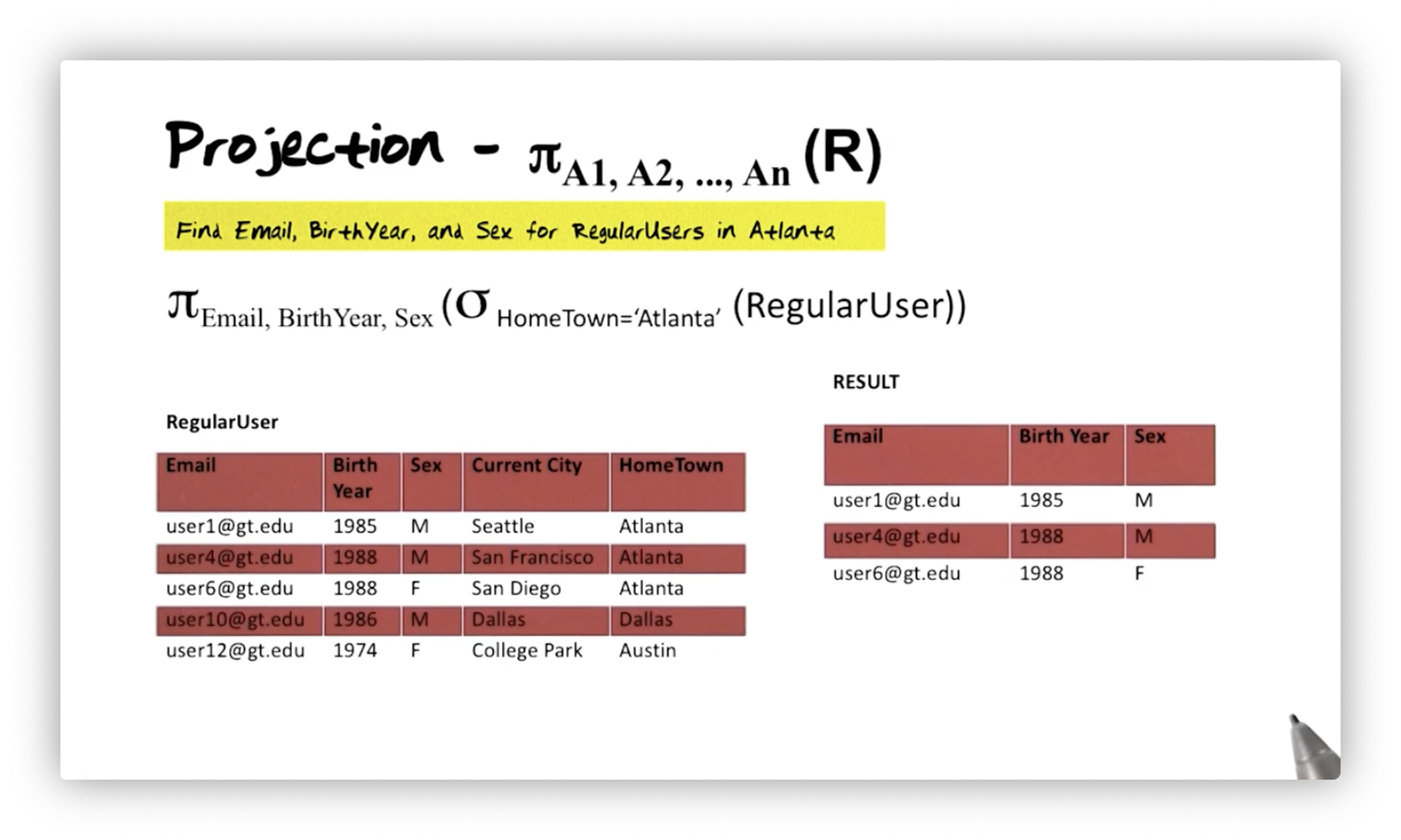
This query demonstrates the power inherent in relational algebra being a closed query language. First, we take the RegularUser relation and perform a selection. From that intermediate result, which we know must be a relation, we can then perform the projection. We can only express composed queries like this when working with a closed algebra.

Relations are Sets

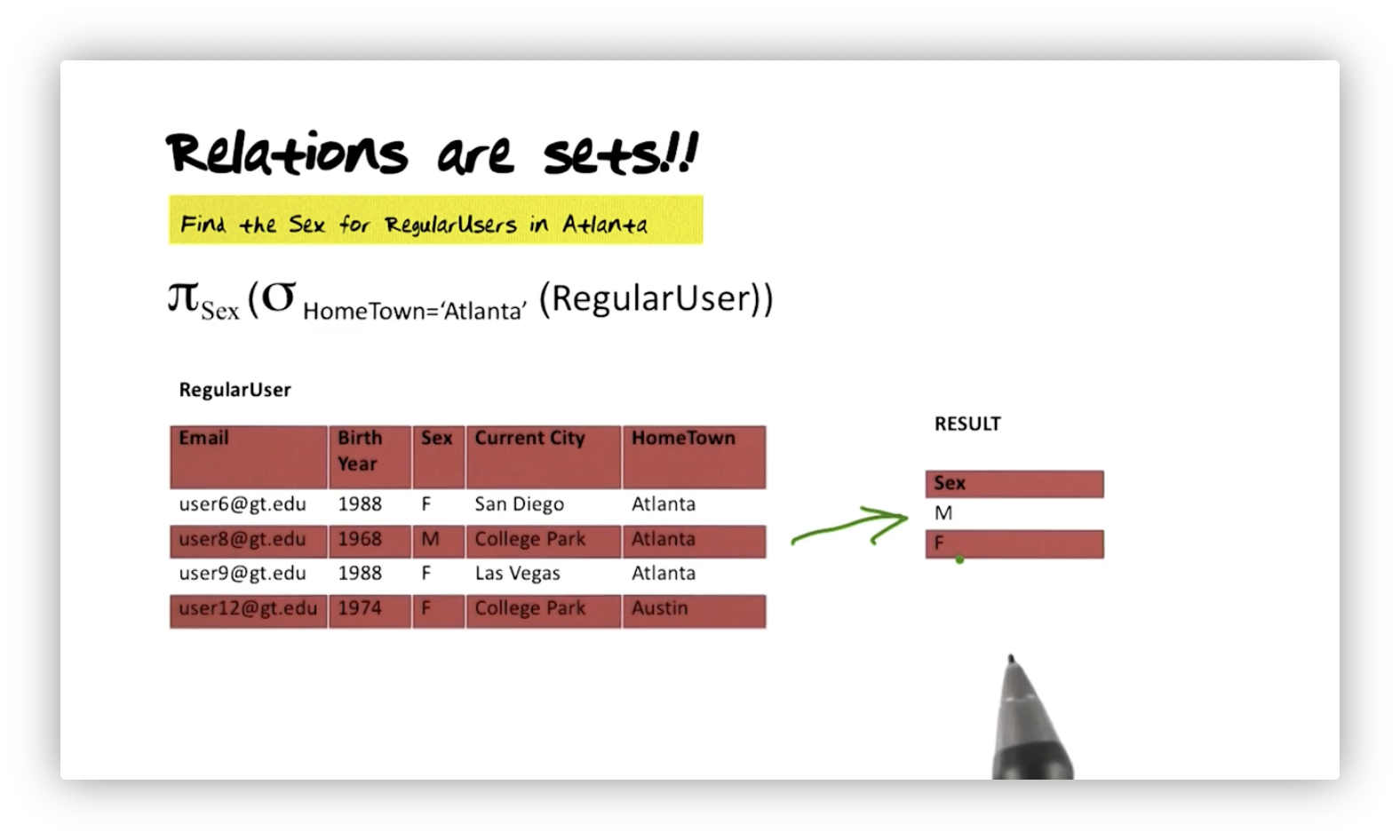
Let's say we want to find the sex of regular users in Atlanta. We could specify that query as:

In the RegularUser table, we have three users from Atlanta, so we have three tuples that match our selection condition. Our projection, however, only shows one "M" and one "F", despite the selection returning two females and one male. In other words, relations are sets and, thus, do not contain duplicate tuples.

Intersection

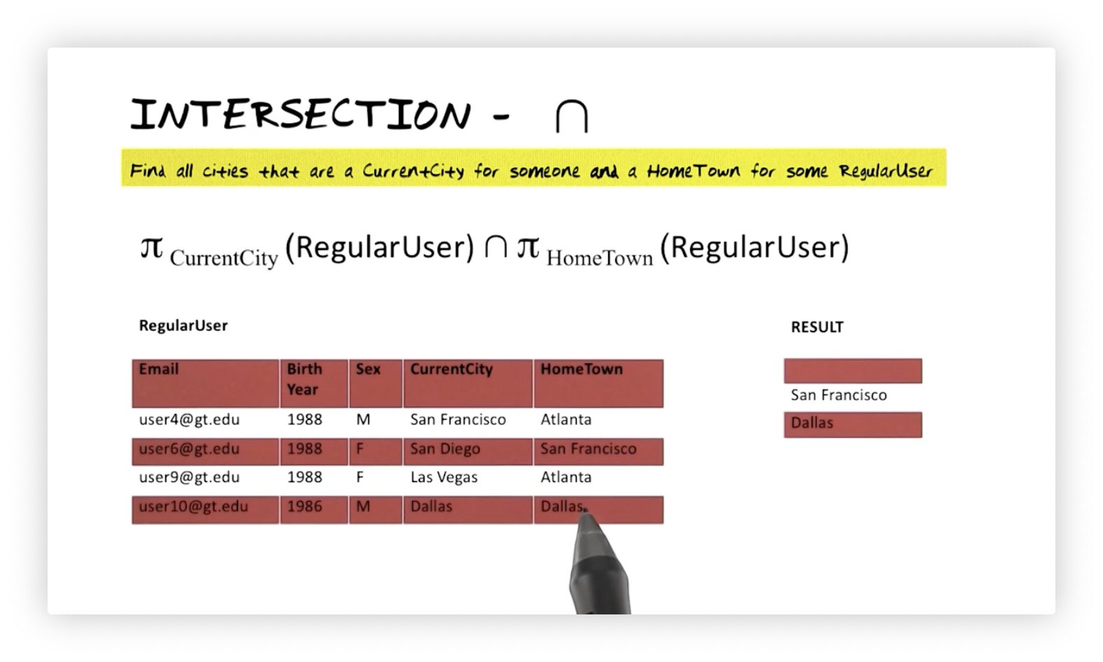
The second set-based operator is the intersection operator: $\cap$. For example, consider the set of cities that are hometowns and the set that are current cities for regular users. We can find the elements that those sets share with the following query:

In the RegularUser relation, we see Dallas and San Francisco appear in both the CurrentCity and HomeTown columns, so those values constitute our result.

Set Difference

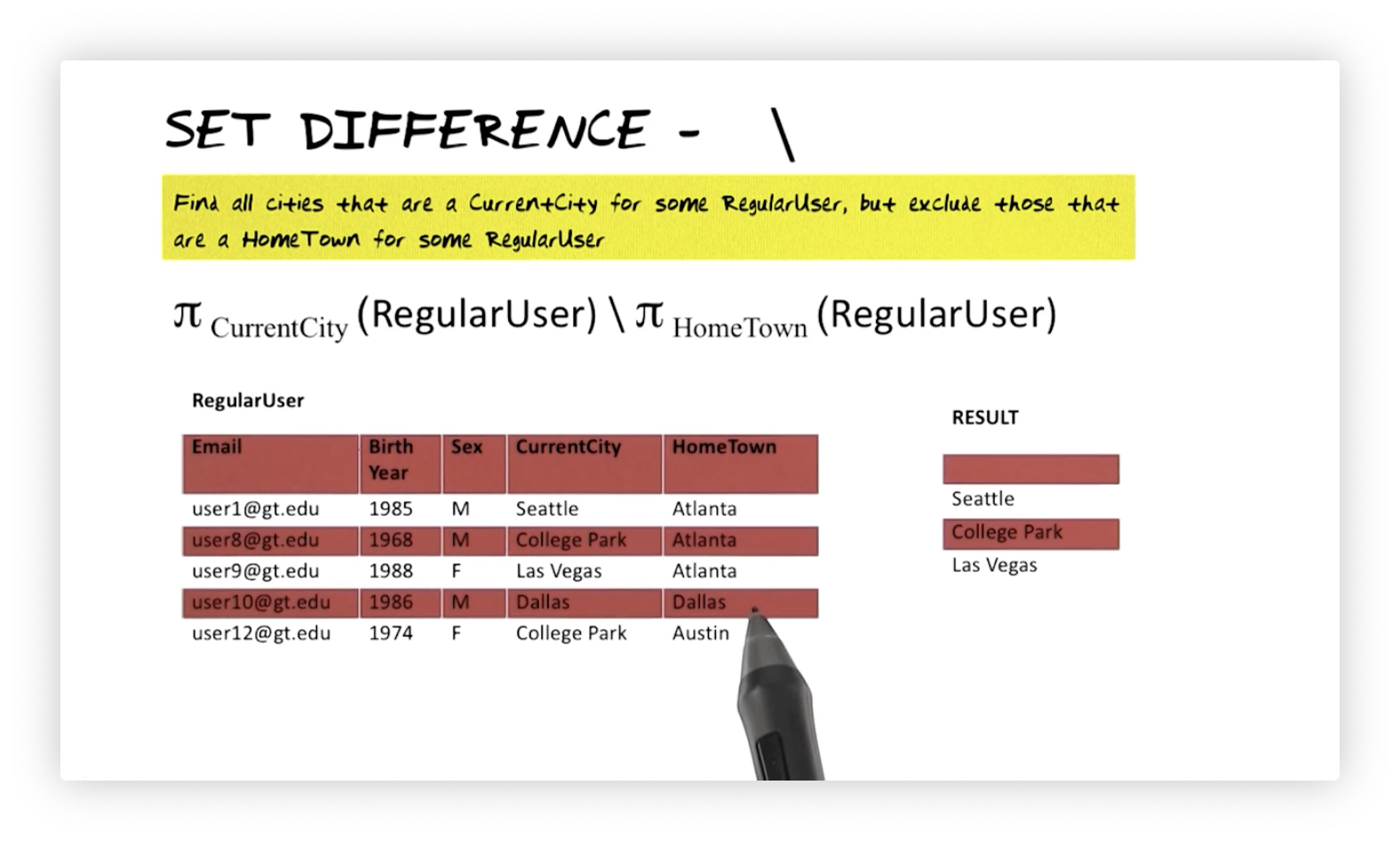
The third set-based operator is the difference operator, $\setminus$. Suppose we want to find the elements of the set of current cities that are not also elements of the set of hometowns. Here's how we would formulate this query:

Of the cities in the CurrentCity column, only Dallas is in the HomeTown column. Thus, we eliminate it from the result. Notice again that we drop duplicate values; College Park appears as a current city twice in RegularUser, but only once in the result.

Natural Join

Let's say we want to generate a relation that displays user and event information for every year an event occurred and a user was born. Suppose we have two relations: RegularUser, with attributes Email, Year, and Sex; and Major60sEvent, with attributes Year and Event. We need to join the two relations to answer this query, and we formalize this natural join as follows:

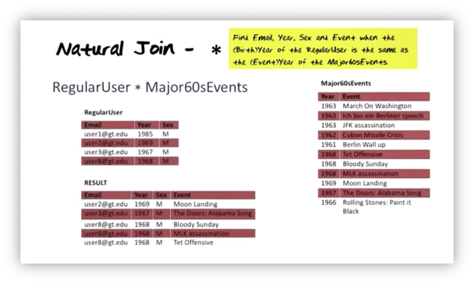
Notice that both RegularUser and Major60sEvents have a similarly named attribute, Year. The natural join operation compares all combinations of tuples from both relations and checks if the value of Year is the same.

If a tuple in either relation has a value of Year that is not present in the other, then that tuple will be absent from the result. In the joined relation, all attributes from the constituent relations are present, with the joined attribute appearing once. If multiple tuples have matching attributes, we will see one tuple in the join relation for each match.

Let's summarize some of the features of a natural join:

• It matches values of attributes with the same name and only those.
• It keeps only one copy of the join attribute in the result.
• We call a natural join an inner joinbecause only the matching tuples appear in the result, with unmatched tuples eliminated.

Theta Join

Next, we look at the theta join. Suppose we want to find the email, birth year, sex, and event year when the birth year of the regular user occurs before the year of the major 60s event. We can formalize this query as follows:

In the result, we see one user born in 1967 predates four events, while another user born in 1968 predates one. Notice that the resulting relation has five rows, not two. Our result has a row for each user/event combination.

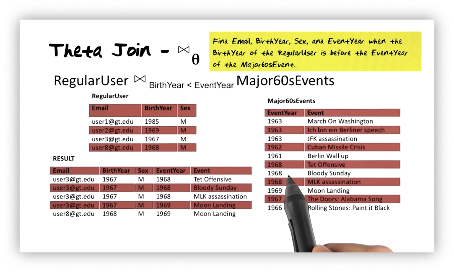
Let's compare the natural join with the theta join:

• A natural join can express only equality conditions, while a theta join can also express inequality conditions using the $<$, $\leq$, $>$, $\geq$, and $\neq$ operators.
• Two relations joined by a natural join must share an attribute name, while the theta join does not have this restriction.
• In the natural join, the join attribute appears once in the result. Both attributes in a theta join appear in the relation (BirthYear and EventYear above).

Like a natural join, a theta join preserves all attributes from the joined relations in the result. The theta join is also an inner join because tuples in the two relations that do not match each other do not appear in the result.

Left Outer Join

The third constructor operator we examine is the outer join operator, specifically the left outer join, whose operator is $\Join_{\text{L}}$. Suppose we want to perform the natural join we saw above and retain unmatched tuples from RegularUser. The algebra expression is:

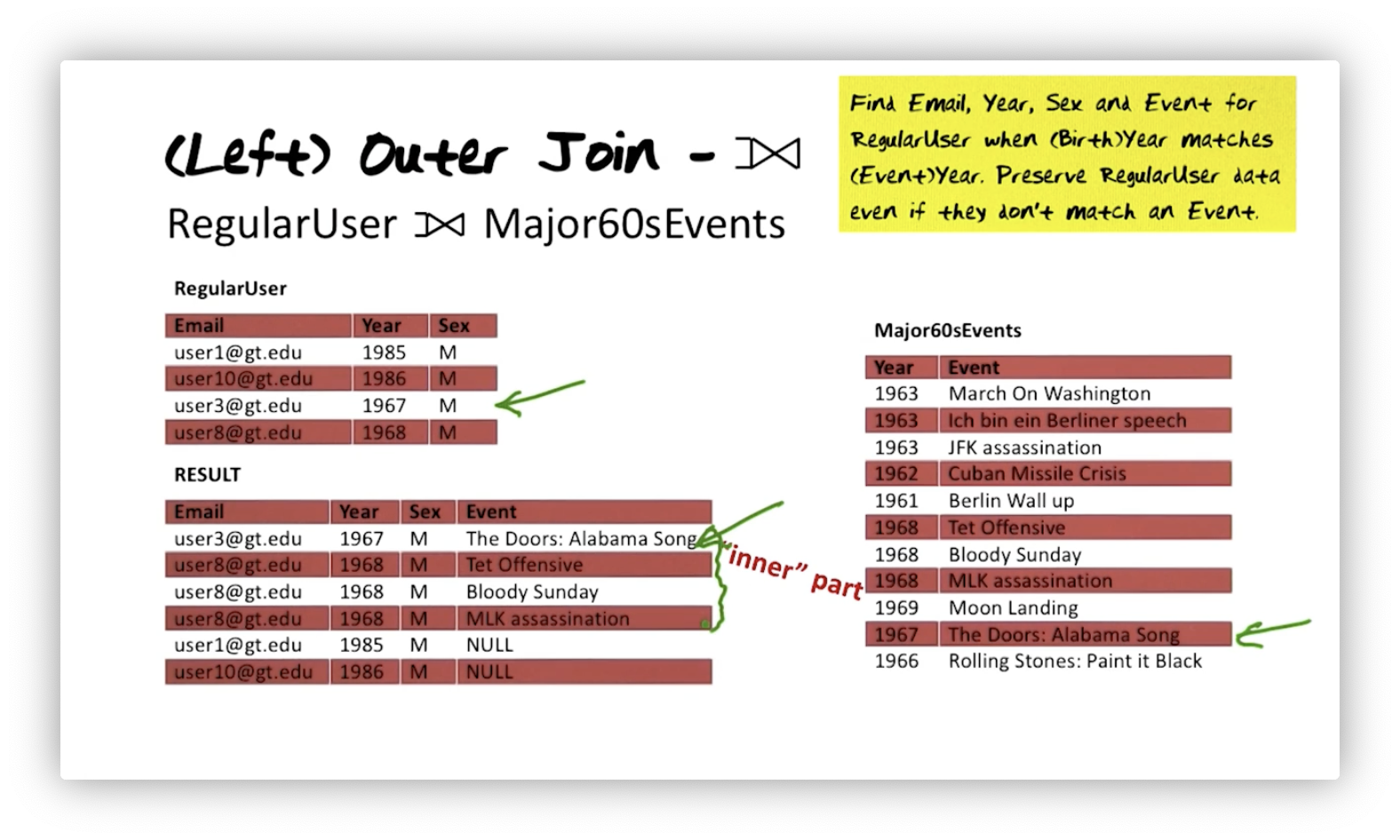
For every user whose birth year matches the event year, we include a tuple for every match. Two users' birth years don't match any event year in the events table. We said we want to retain their information, and we can include it, but we must fill in the absent event information with NULL values. That NULL corresponds to the "outer" part of the result.

The resulting relation is a superset of the result of the natural join we expressed earlier. In this case, the left outer join we saw here is a natural left outer join - a special case of the natural join - because we compared attributes of the same name.

Cartesian Product: X

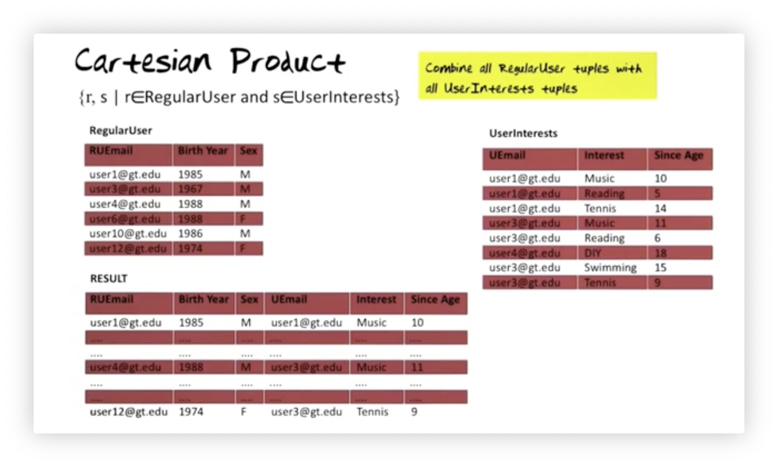
The fourth constructor operator in the relational algebra is the Cartesian product operator, $\times$. A Cartesian product, $A \times B$, results in a relation with $N * M$ tuples, where $N$ is the number of tuples in $A$, and $M$ is the number of tuples in $B$. For example, we can combine every tuple in RegularUser with every tuple in UserInterests:

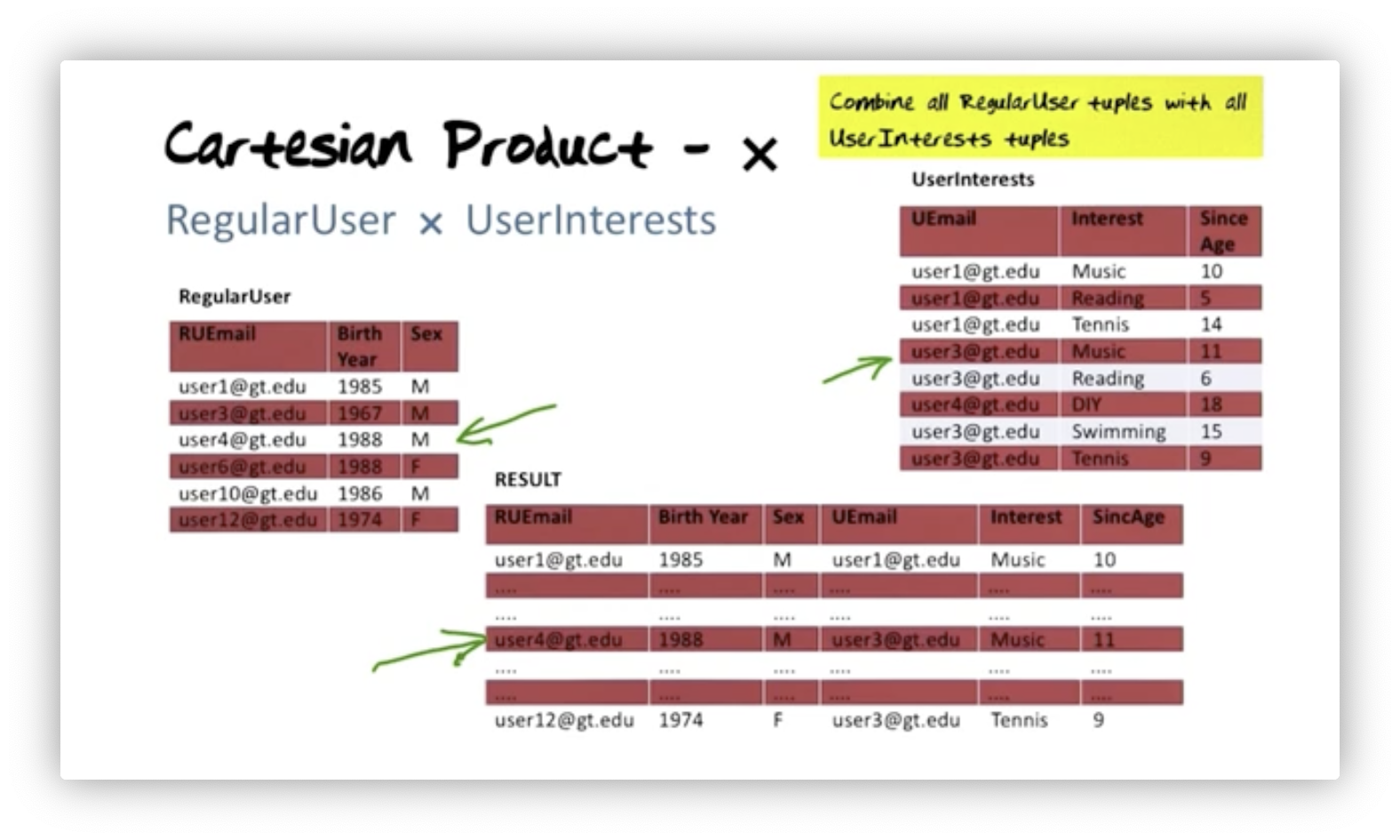
There are no comparison rules in the Cartesian product - in contrast to the other joins - to selectively include only certain matches in the result. Here, we combine everything. Why might that be useful?

Cartesian Product: Can be Useful

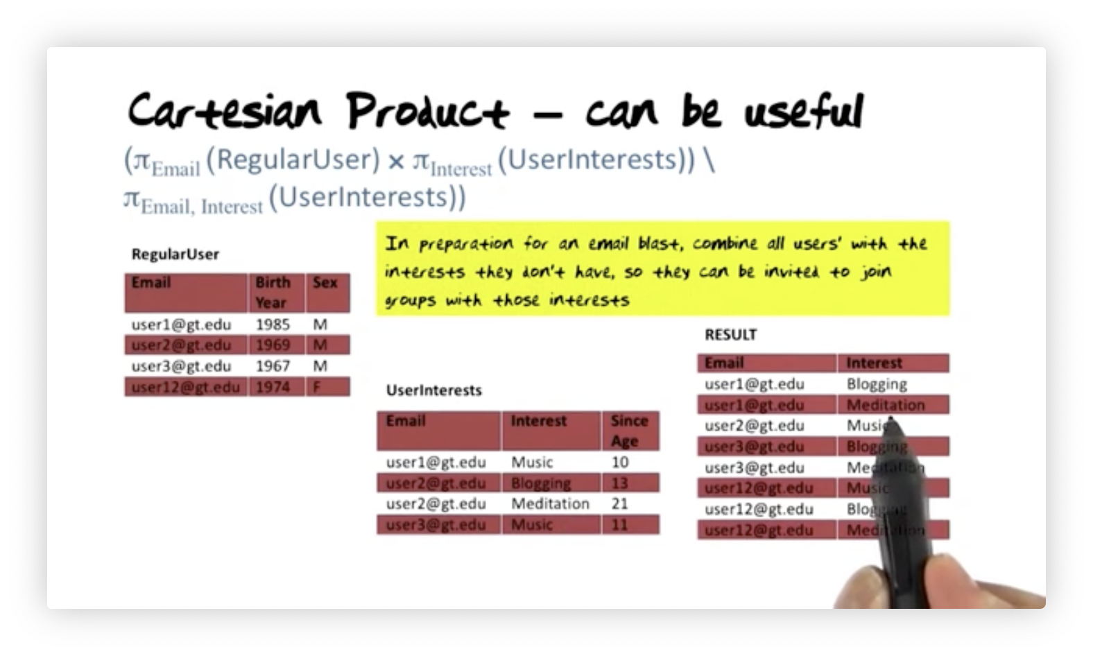
Suppose we have a RegularUser relation and a UserInterests relation. The UserInterests table contains information about users' interests and has a foreign key, Email, that references the primary key in RegularUser. We want to find all the hobbies in which each user has not expressed interest.

First, we project RegularUser onto Email and UserInterests onto Interest so that we have one relation containing just user emails and another with just user interests. Now, we compute the Cartesian product of the two results, which creates a tuple for each user for each interest. Finally, we subtract from this result UserInterests to eliminate the interests we already recorded. We express this query as:

Notice that the two operands in the set difference are compatible. The resulting relation from the Cartesian product operation has Email and Interest attributes, and from that, we subtract the projection of UserInterests onto Email and Interest (dropping Since Age).

Here is the result. Let's look at user one, for example. In UserInterests, this user has music as an interest but not blogging or meditation. We see those two hobbies associated with this user in the result.

Divide By

Now let's look at the divide by algebra operator: $\div$. This operator plays the same role in relational algebra as universal quantification in relational calculus. Suppose we want to find the email of all users with at least all the interests of user one.

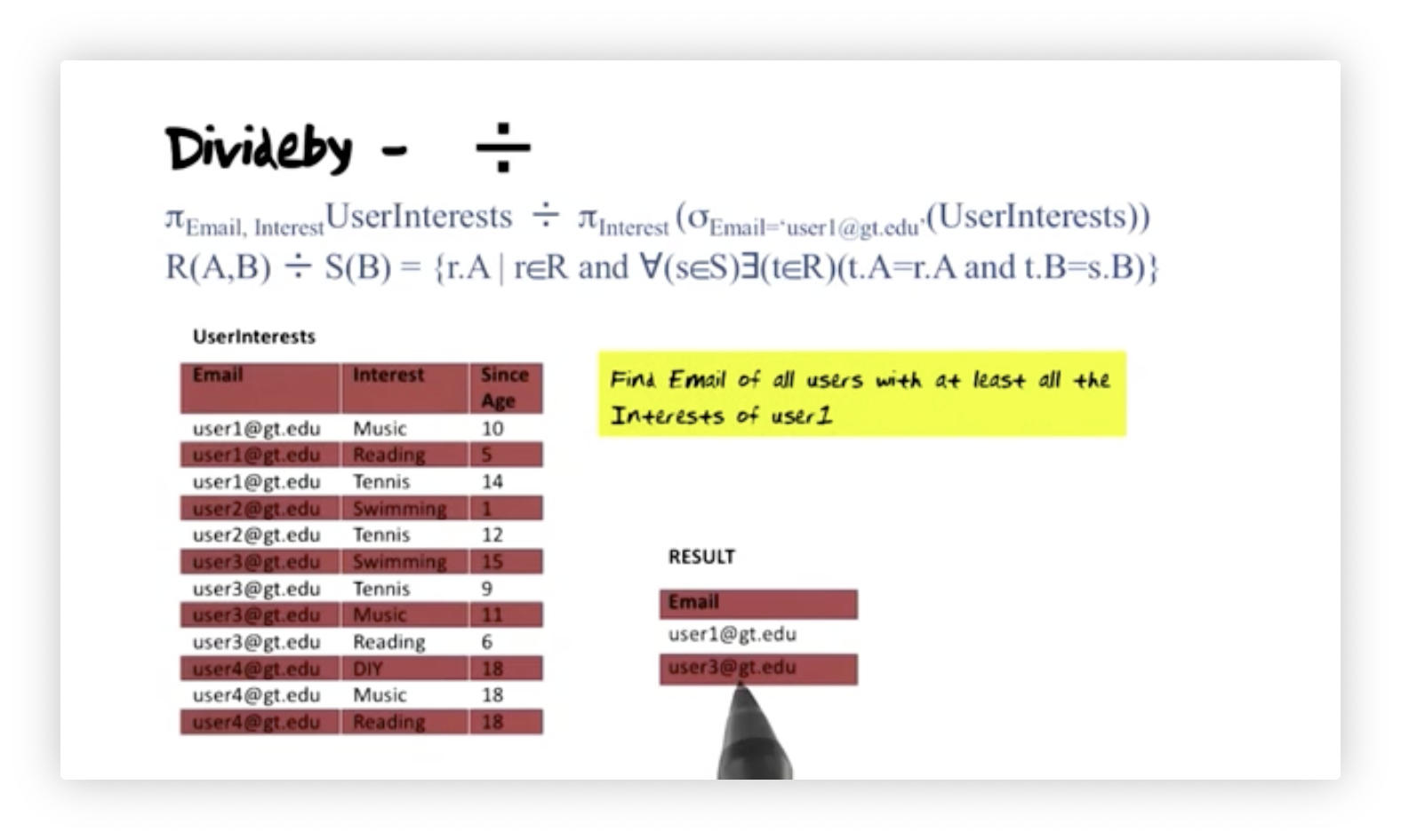
User one has three interests: music, reading, and tennis. User one has at least as many interests as user one, so we include them in the result. User three has all of the interests of user one plus more, so we include them in the result too. Neither user two nor user four have at least the set of interests that user one has, so they are absent from the result.

Here's how we perform the divide-by operation. First, we calculate the divisor by projecting UserInterest onto Email and Interest. Then, we calculate the dividend by selecting user one's interests from UserInterest and then projecting that relation onto Interest. The result is a single-column relation containing music, reading, and tennis. We can express this query in the algebra like so:

When we divide one relation by another, the divisor has attributes $A$ and $B$, the dividend has attribute $B$, and the result has attribute $A$. We divide $\text{Email, Interest}$ by ${\text{Interest}}$ to produce $\text{Email}$ here. The divide by operation always follows this structure.

Here is formal definition of the result where $\text{R}$ is the RegularUser relation, $\text{S}$ is the intermediate projection of user one's interests, $\text{E}$ is short for "Email" and $\text{I}$ is short for "Interest":

What this formalism describes is the following. Let's look at each candidate tuple $\text{r}$ in relation $\text{R}$. For all ($\forall$) tuples $\text{s}$ in relation $\text{S}$, if there exists ($\exists$) a tuple $\text{t}$ in $\text{R}$ such that $\text{t}$ and $\text{r}$ have the same email and $\text{t}$ and $\text{s}$ have the same interest, then include $\text{r.Email}$ in the result.

Rename

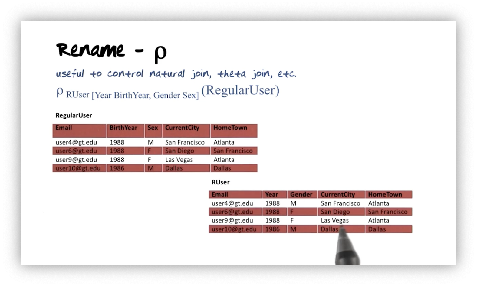
The last algebraic operator we examine is the rename operator, $\rho$. Renaming attributes and relations is useful when we want to perform various types of joins. Here is the basic syntax:

For example, we can rename the RegularUser relation to RUser, the BirthYear attribute to Year, and the Sex attribute to Gender:

Relational Calculus

Relational algebra is procedural; we combine operators to describe the steps we must take to produce the desired result. For instance, we might say join two relations, project the result, and then select from that result to get the final relation. Relational calculus is declarative. Instead of describing steps, we describe the result we want. Relational tuple calculus forms the basis of SQL.

One might think that tuple calculus has more expressive power than algebra. As it turns out, both can be shown to be equivalent regarding data retrieval "horsepower", as Professor Mark calls it.

Relational Calculus Expressions

Let's look at expressions in relational calculus - specifically relational tuple calculus, so named because queries have variables that range over sets of tuples. Here's a query:

This query returns the set of tuples $\text{t}$ that satisfy the predicate $\text{P}$. Predicates consist of atoms, so let's first define the atoms in this calculus.

The first atom is the range expression. For example, $\text{t} \in \text{R}$, and $\text{R(t)}$ denote that $t$ is a tuple of relation $R$. The second atom compares two tuple attributes. We reference tuple attributes as follows: $\text{t.A}$ denotes the value of attribute $\text{A}$ on tuple $\text{t}$. The third atom compares a tuple attribute to a constant, $\text{c}$. We use $\theta$ to denote comparison operators, which consist of $<$, $\leq$, $>$, $\geq$, and $\neq$.

In summary, atoms are one of the following:

• A range expression: $\text{t}\in \text{R}$
• A comparison of two attributes: $\text{r.A } \theta \text{ s.B}$
• A comparison of one attribute and a constant: $\text{r.A } \theta \text{ c}$.

An atom is a predicate. Furthermore, given atoms $\text{P}_1$ and $\text{P}_2$, the following expressions are also predicates: $(\text{P}_1)$, $\text{not P}_1$, $\text{P}_1 \text{ or } \text{P}_2$, $\text{P}_1 \text{ and } \text{P}_2$, and $\text{P}_1 \implies \text{P}_2$, where $\implies$ means "implies".

Finally, if $\text{P(t)}$ is a predicate and ${\text{t}}$ is a free variable in $\text{P}$, and $\text{R}$ is a relation, then "there exists a $\text{t}$ in $\text{R}$ that satisfies $\text{P}$" is a predicate called the existential quantifier: $\exists (t\in R)(P(t))$. Likewise, "for all $\text{t}$ in $\text{R}$ for which $\text{P(t)}$ is true" a predicate called the universal quantifier: $\forall \text{(t } \in \text{R)(P(t))}$. If $\text{t}$ is free in the predicate $\text{P}$, then using the existential quantifier or the universal quantifier binds $\text{t}$.

Calculus - Selection

For the rest of the lectures in this section, we will revisit the queries we saw in the relational algebra section and express them using relational tuple calculus. Here is the corresponding tuple calculus expression for selecting all regular users:

We can think of this query as: find the set $\text{r}$ where $\text{r}$ is a member of the relation $\text{ RegularUser\}}$. As we might expect, this relation is identical to $\text{ RegularUser}$.

Calculus - Selection: Composite Expression

Let's find all regular users who have the same current city and hometown or have a hometown of Atlanta:

Notice that even if we had another relation with the attributes CurrentCity and HomeTown with similar values, those tuples would be absent from the result because they did not come from $\text{RegularUser}$. All expressions in the selection query must be true for a tuple to appear in the result.

Calculus - Projection

Suppose we want to find the email, birth year, and sex for all regular users whose hometown is Atlanta. Here is that query:

We can see below that the resulting relation consists of only the requested attributes for the tuples that match the selection query.

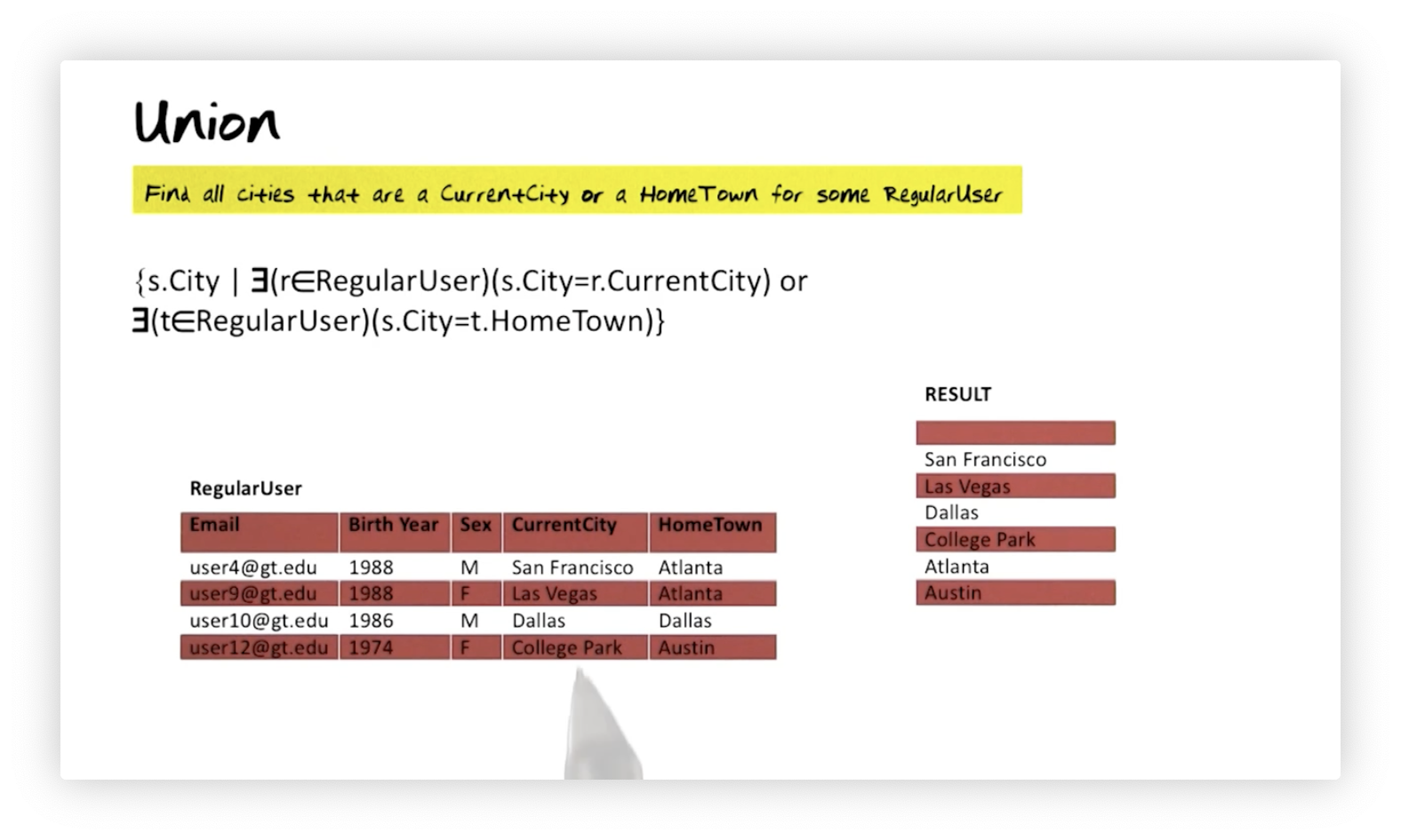
Calculus - Union

Let's find all cities that are either a current city or a hometown for a regular user.

If a tuple exists in $\text{RegularUser}$ with a current city, then that city is part of the result. Similarly, if a tuple exists in $\text{RegularUser}$ with a hometown, then that city is part of the result.

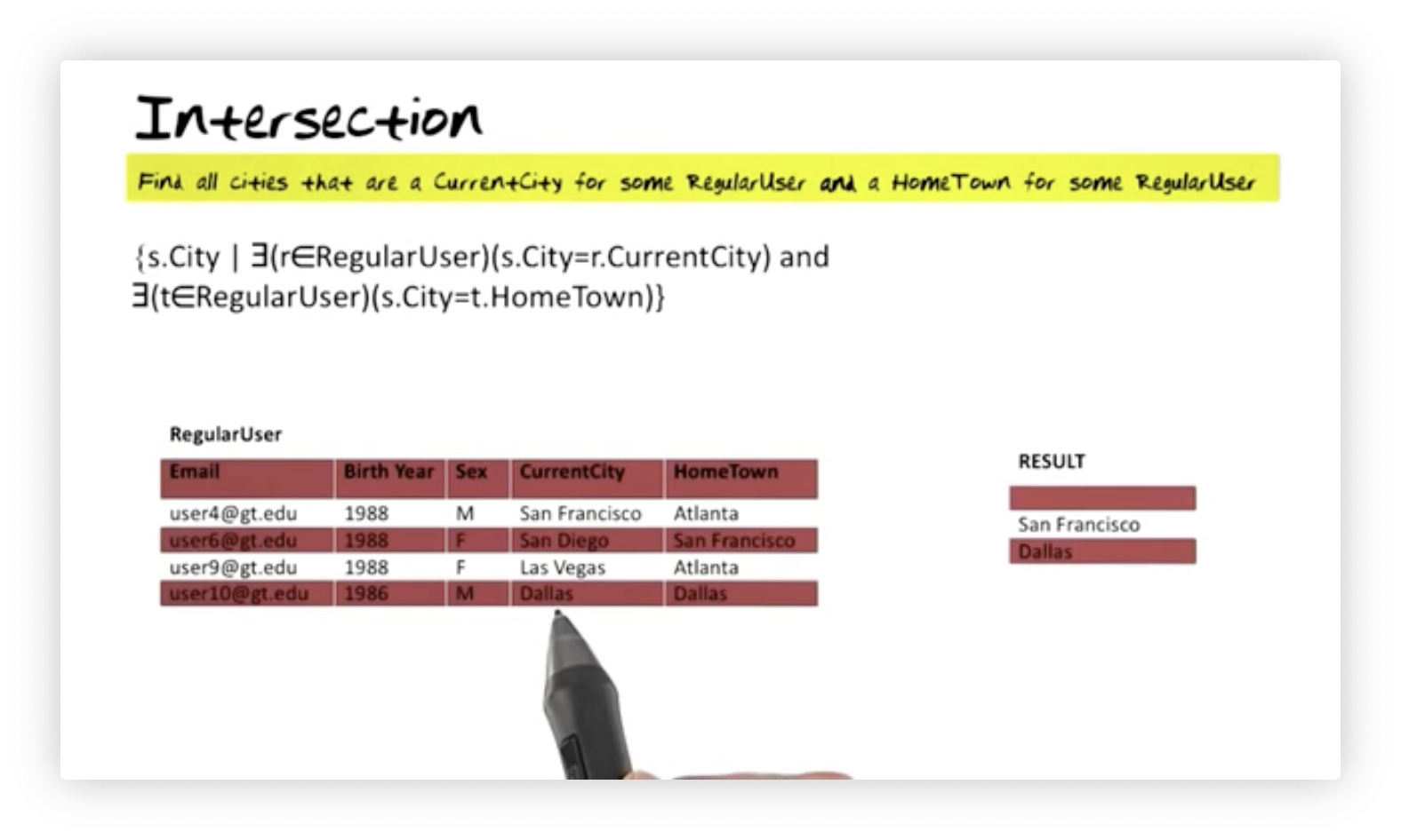
Calculus - Intersection

Let's find all cities that are a current city for some regular user and a hometown for some regular user.

For a tuple $\text{s}$ to qualify, there must exist a tuple $\text{r}$ in $\text{Regular User}$ that has the same city as $\text{s}$, and it must also be the case that there is a tuple $\text{t}$ that has the same hometown as $\text{s}$. We retrieve the $\text{City}$ attribute for qualifying tuples.

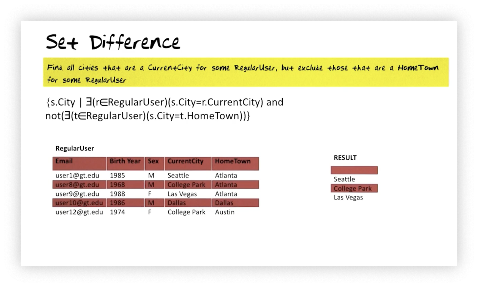
Calculus - Set Difference

Suppose we want to find the elements of the set of current cities that are not also elements of the set of hometowns. Here's how we would formulate this query:

For a tuple $\text{s}$ to qualify, there must exist a tuple $\text{r}$ in $\text{Regular User}$ that has the same city as $\text{s}$, and it must also be the case that there is not a tuple $\text{t}$ that has the same hometown as $\text{s}$. We retrieve the $\text{City}$ attribute for qualifying tuples.

Calculus - Natural Join

Let's say we want to generate a relation that displays user and event information for every year an event occurred and a user was born. Suppose we have two relations: $\text{RegularUser}$, with attributes $\text{Email}$, $\text{Year}$, and $\text{Sex}$; and $\text{Major60sEvent}$, with attributes $\text{Year}$ and $\text{Event}$. We need to join the two relations to answer this query, and we formalize this natural join as follows:

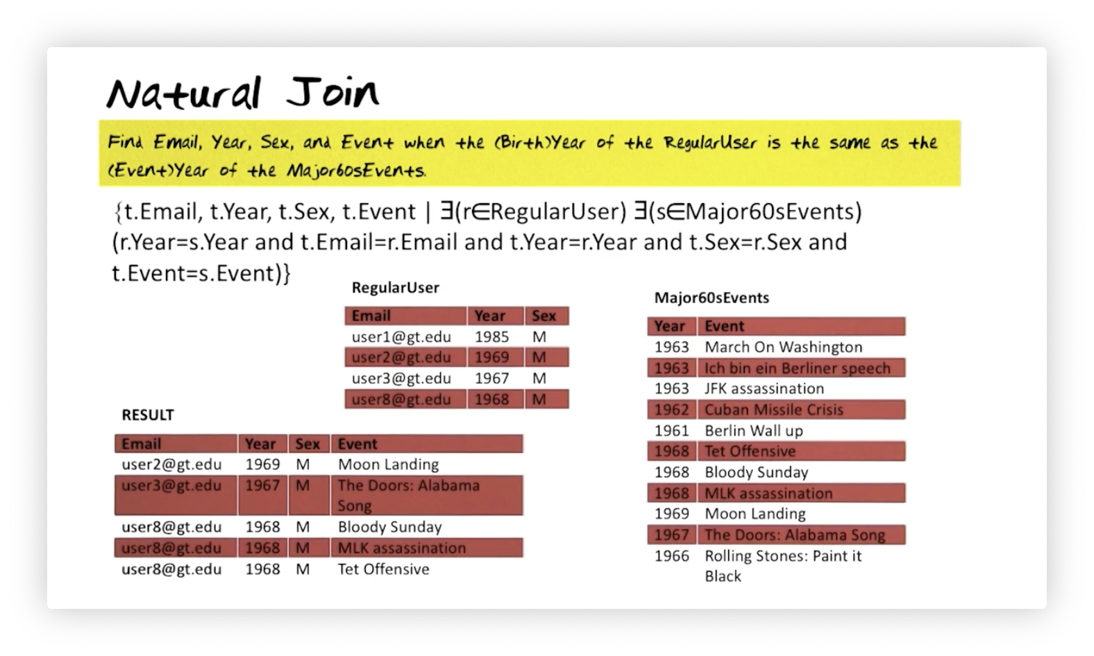
Let's decipher this query expression. We are interested in a tuple, $\text{t}$ that contains $\text{Email}$, $\text{Year}$, $\text{Sex}$, and $\text{Event}$ attributes. What must be true for us to include $\text{t}$ in the result? Well, there must exist a tuple $\text{r}$ in $\text{RegularUser}$ and a tuple $\text{s}$ in $\text{Major60sEvent}$. If $\text{r.Year}$ equals $\text{s.Year}$, then we pick $\text{r.Email}$, $\text{r.Year}$, $\text{r.Sex}$, and $\text{s.Event}$ into $\text{t}$ and include it in the result.

Calculus - Cartesian Product

Let's say we want to combine every tuple in the $\text{RegularUser}$ relation with every tuple in the $\text{UserInterests}$ relation. We can express that Cartesian product in relational calculus like so:

Calculus - Cartesian Product: Can be useful

Suppose we have a $\text{RegularUser}$ relation and a $\text{UserInterests}$ relation. The $\text{UserInterests}$ table contains information about users' interests and has a foreign key, $\text{Email}$, that references the primary key in $\text{RegularUser}$. We want to find all the hobbies in which each user has not expressed interest. Here is how we express this query:

We are looking for a tuple, $\text{r}$, from $\text{RegularUser}$ and a tuple, $\text{s}$, from $\text{UserInterests}$ where it is not the case that there exists a tuple, $\text{t}$, from $\text{UserInterests}$ that has the same $\text{Email}$ as $\text{r}$ or the same $\text{Interest}$ as $\text{s}$. We then select $\text{r.Email}$ and $\text{s.Interest}$ for those tuples $\text{r}$ and $\text{s}$ for which this predicate is true.

Calculus - Divide By

Suppose we want to find the email of all users with at least all the interests of user one. Here is how we express that query in relational calculus:

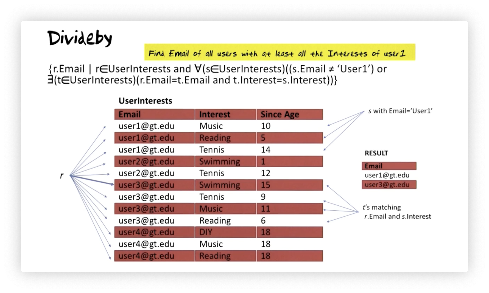
We are interested in values of the $\text{Email}$ attribute on tuples $\text{r}$ from the $\text{UserInterests}$ relation. For a candidate $\text{r}$ tuple, we must check that something is true for every tuple $\text{s}$ in $\text{UserInterests}$. Either the value of the $\text{Email}$ attribute for $\text{s}$ must not be user one's email address, or, if it is, then the following must be true: there must exist a tuple $\text{t}$ in $\text{UserInterests}$ that shares an email with $\text{r}$ and an interest with $\text{t}$.