Localization Overview

Localization

Suppose we are driving a car on a highway, and we'd like to know where we are. These days, many cars and cellphones have applications that interact with the global positioning system, GPS. After receiving a few satellite signals, these apps can show us cruising along as little dots on virtual maps.

Now suppose we are building a self-driving car. Just like a human driver, a robot driver needs to understand where it is within the world. Is it driving inside the lane markers, or is it veering off a cliff?

Localization is the process by which the robot establishes its position in the world.

A self-driving car might need to localize on several different scales. For example, to know if it has arrived in its destination city, the car might use GPS.

If the car needs to determine whether it is driving within lane markers, however, GPS is a terrible choice. The margin of error for GPS is 10 meters, which is roughly the width of three highway lanes in the United States. For self-driving cars to be able to stay in lanes using localization, we need a margin of error on the order of magnitude of 2-10cm.

Total Probability

Let's begin our story with a robot. This robot lives in a world, but, alas, it has no idea where it is in the world.

We can represent the robot's understanding of its current location in the world with a probability distribution, $P(X)$, where $X$ is a location in the world, and $P(X)$ represents the probability that the robot is currently at location $X$.

The probability distribution that our robot starts with - assuming no prior knowledge - is a discrete uniform distribution. In other words, the robot is equally likely to be in any of the $n$ locations in the world, each with a probability of $\frac{1}{n}$.

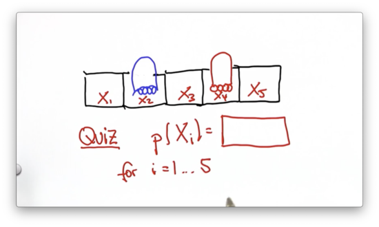
For localization to be possible, the world has to have some distinctive features. Let's assume that there are three different landmarks in the robot's world: the three doors drawn below.

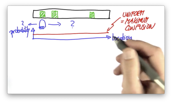
Let's also assume that the robot cannot distinguish one door from another but can distinguish a door from a "non-door".

Now suppose that the robot "open its eyes" and senses that it is standing next to a door. This measurement transforms our discrete uniform distribution - the "naive" understanding - into a new probability distribution that looks like this.

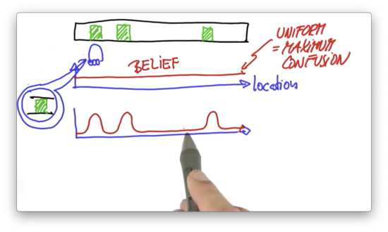
Relative to the previous understanding of the world, this new understanding associates a higher probability to locations adjacent to doors and a lower probability to all other locations. We refer to this belief about the world as a posterior belief, as it was formed after a measurement was taken.

One key aspect of this belief is that the robot still doesn't know where it is; after all, there are three doors. On top of that, we can't rule out the possibility that the sensors are erroneous and the robot saw a door where there was none. While these three bumps express the robot's best belief about where it is, there is a residual probability that the robot is in a non-door location.

Now let's assume the robot moves to the right by a certain distance. We can shift our belief according to the motion. Technically, this "shifting" operation is known as a convolution.

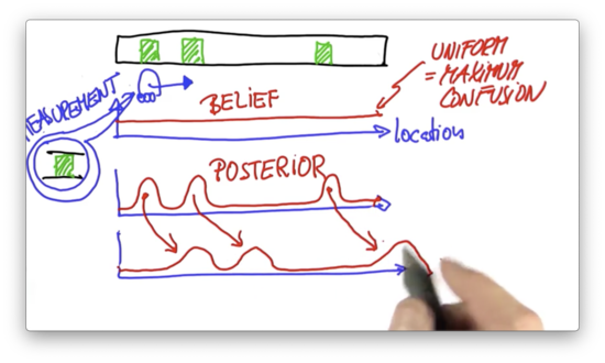
The robot knows both the direction and magnitude of its movement. Robot motion is somewhat uncertain, however, so the shifted probability distribution has peaks that are shorter and wider.

Assume that the robot senses again, and it senses that it is right next to a door. To obtain our second posterior belief, we multiply our shifted probability distribution with a distribution that looks very similar to our first posterior belief; that is, a distribution with high probabilities at locations associated with doors.

In this second posterior belief, the only significant probability peak corresponds to the position of the second door. From the three locations associated with relatively high probability in the prior belief, only one of them corresponds to a door. As a result, this posterior belief amplifies the prior peak associated with the door while effectively muting the other prior peaks.

At this point, our robot has localized itself.

Uniform Probability Quiz

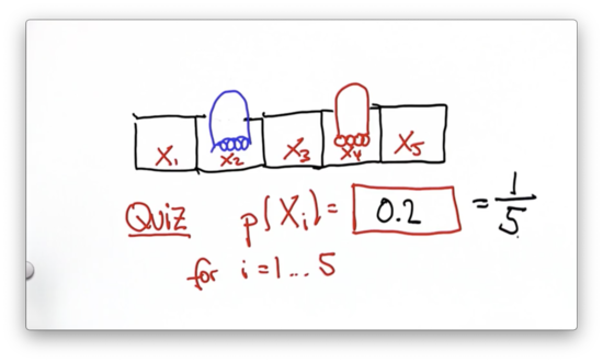
Consider a robot in a world made up of five cells. The robot is equally likely to occupy any one of the five cells. If we select a cell at random, what is the probability that the robot is occupying that cell?

Uniform Probability Quiz Solution

Uniform Distribution Quiz

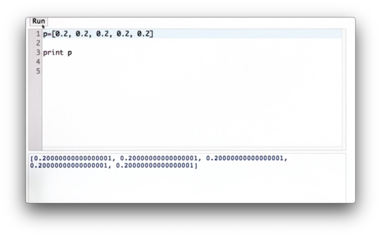
Consider a robot in a world made up of five cells. The robot is equally likely to occupy any one of the five cells. Can we modify the list, p, below to represent the discrete uniform distribution that describes the probability of finding the robot in each of the five cells?

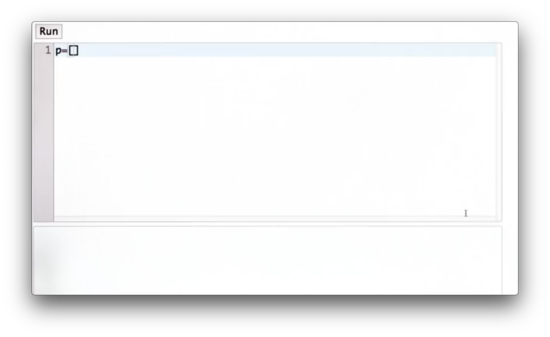
Uniform Distribution Quiz Solution

Generalized Uniform Distribution Quiz

Let's assume that we don't know the dimensions of the world ahead of time. Given a variable, n, representing the number of cells in the world, let's write some code to create a list representing the discrete uniform distribution parameterized by n.

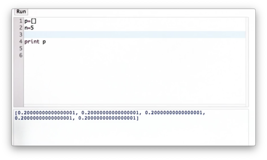
Generalized Uniform Distribution Quiz Solution

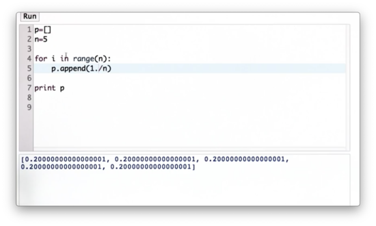
Note that if we used 1 instead of 1. in the numerator, we would have a list of zeros because the / operator performs integer division in Python 2.7. In Python 3+, this casting is unnecessary as / performs float division.

Alternatively, we can use a list comprehension to create p:

p = [1. / n for _ in range(n)]

If that wasn't terse enough, this is also valid.

p [1. / n] * n

Probability After Sense Quiz

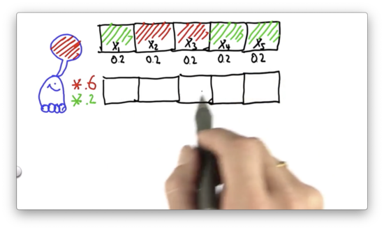
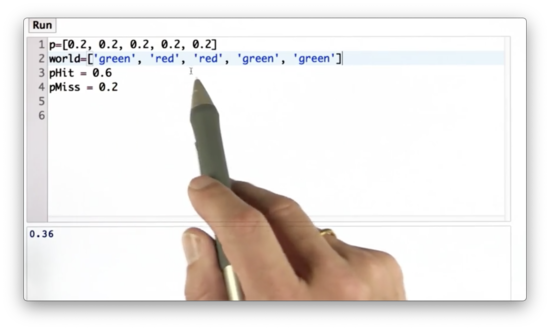
It's time to add some color to our five-celled world. Let's assume that two of the cells in this world are colored red, whereas the other three are green.

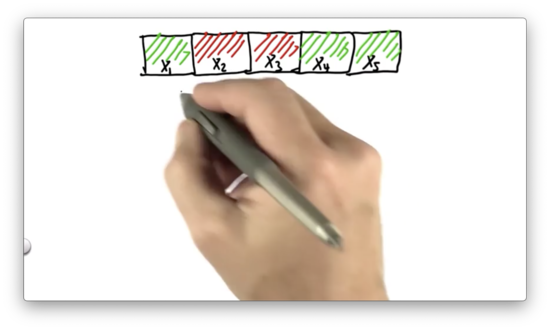
As before, we assign a uniform probability of 0.2 to each cell. Now let's assume we allow our robot to sense, and it sees a red color.

How will this affect the robot's belief about where it is located? Intuitively, the probabilities associated with $x_2$ and $x_3$ should increase while the probabilities associated with $x_1$, $x_4$, and $x_5$ should decrease.

We can incorporate this measurement of "red" into our belief using a product. We can multiply the current probability associated with a cell by a large number - say, 0.6 - when the color of the cell is red. Similarly, we can multiply the current probability associated with a cell by a small number - say, 0.2 - when the color of the cell is green.

Looking at the ratio between these two factors, 0.2 and 0.6, we can see that our posterior belief is going to assign probabilities to red cells that are three times larger than those associated with green cells.

For each of these five cells, what is the resulting probability if we apply this update rule?

Probability After Sense Quiz Solution

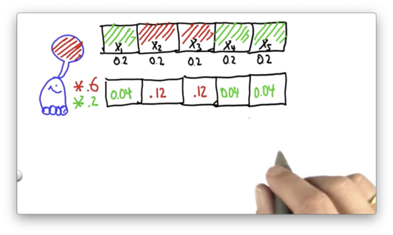
We multiply each green cell by 0.2 and each red cell by 0.6. Each red cell becomes 0.04, while each green cell becomes 0.12.

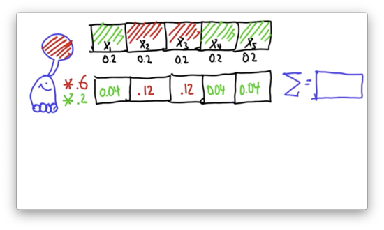
Compute Sum Quiz

In principle, this new probability function is our next belief. The only problem is that it's not a valid probability distribution because the probabilities do not add up to 1. What is the sum of these probabilities?

Compute Sum Quiz Solution

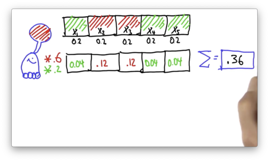
Normalize Distribution Quiz

To turn this probability function into a probability distribution, we normalize the individual probabilities by dividing them by 0.36. What are the normalized values?

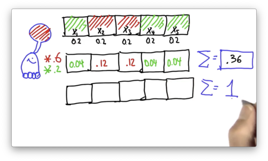
Normalize Distribution Quiz Solution

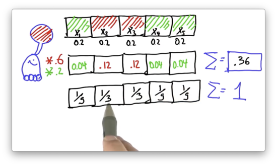
If we divide 0.12 by 0.36, we get $\frac{1}{3}$. If we divide 0.04 by 0.36, we get $\frac{1}{9}$. The sum of the five probabilities shown above equals 1, which indicates that we have a valid probability distribution.

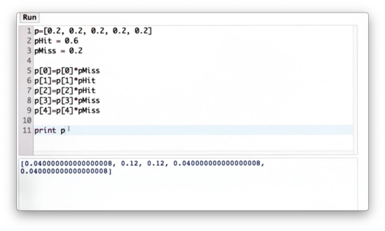
pHit and pMiss Quiz

Let pHit be the factor by which we multiply cells that match our measurement, and pMiss be the factor by which we multiply cells that don't match our measurement. Our task is to write code that outputs the non-normalized posterior probability distribution, using p, pHit, and pMiss, given that positions $x_2$ and $x_3$ are hits.

pHit and pMiss Quiz Solution

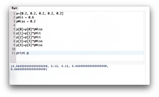
We can explicitly multiply each value by pHit or pMiss depending on its index. This solution is not particularly elegant.

Alternatively, we could use the enumerate function in Python:

for idx, prob in enumerate(p):
    if idx in [1,2]:
        p[idx] *= pHit
    else:
        p[idx] *= pMiss

Sum of Probabilities Quiz

Since we need the sum of the probabilities to normalize them, let's write some code to compute the sum of the values in p.

Sum of Probabilities Quiz Solution

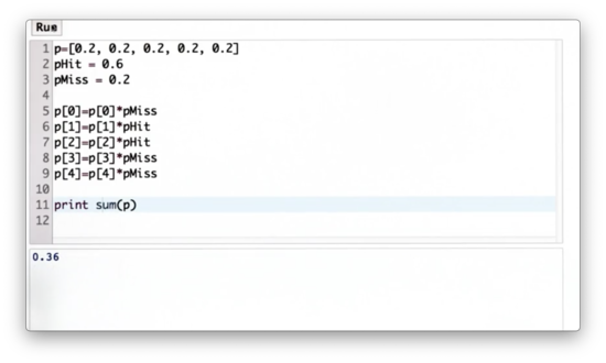
We can use the builtin sum function to sum the elements in p.

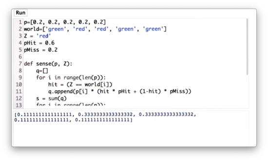
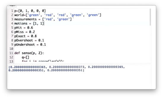
Sense Function Quiz

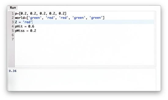
Let's make this code a little bit better. First, we are going to introduce a variable, world, which is a list of the colors of the cells in the robot's one-dimensional world.

Further, we can define a measurement, Z, to be '"red".

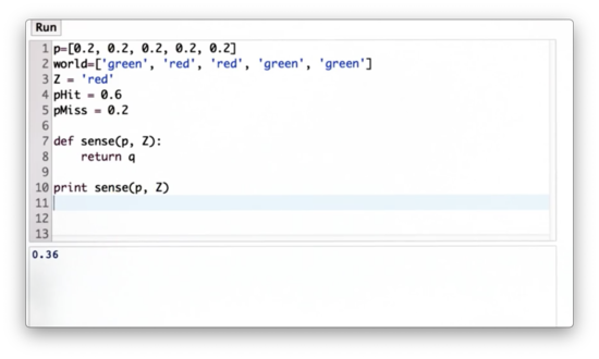
Now let's define a function, sense, which takes as input the initial distribution, p, and the measurement, Z, and outputs the normalized distribution, q. q reflects the non-normalized posterior belief created by multiplying the appropriate elements in p by pHit or pMiss in accordance with Z and the corresponding elements in world.

Our task is to implement sense.

Sense Function Quiz Solution

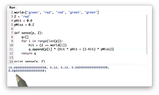
Alternatively, we can use the zip function to combine p and world and make our lives a little bit easier:

def sense(p, Z):
    q = []

    for pi, loc in zip(p, world):
        q.append(pi * (pHit if Z == loc else pMiss))

    return q

If we want to get real fancy, we can even one-line it:

def sense(p, Z):
    return [pi * (pHit if Z == loc else pMiss) for pi, loc in zip(p, world)]

Normalized Sense Function Quiz

Let's modify the sense function to return a valid probability distribution. We need to normalize the values in q so that they add up to 1.

Normalized Sense Function Quiz Solution

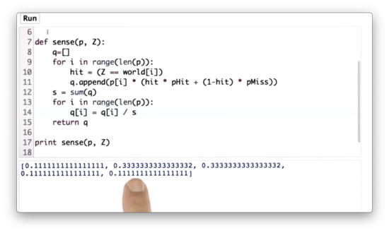
We can compute the sum of q using the sum function and then divide each value in q by that sum. With that, we've implemented the critical function of localization, which is called the measurement update.

Test Sense Function Quiz

What happens if our measurement is "green" instead of "red"? Let's change the value of Z to "green" and see how our new posterior distribution looks.

Test Sense Function Quiz Solution

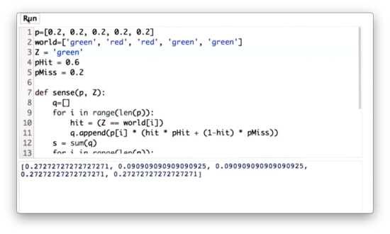
We can see that the first, fourth, and fifth values have a much larger value than the second and third; in fact, three times larger.

Multiple Measurements Quiz

Let's modify the code now to support multiple measurements. Instead of using Z to represent a single measurement, let's create a list of measurements, measurements.

Our task is to write some code that uses measurements and sense to return the posterior probability distribution after multiple measurement updates.

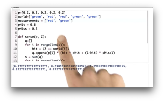
Multiple Measurements Quiz Solution

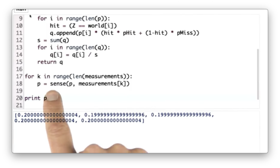
Since sense takes in a probability distribution and a measurement and returns a probability distribution, we can simply iterate over all the measurements in measurements and continuously transform the original distribution p on each iteration.

Exact Motion Quiz

Before we finish with localization, let's talk about robot motion. Suppose we have the following probability distribution associated with the five cells in our world.

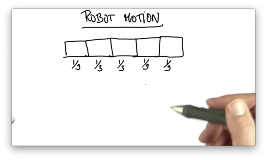
Suppose we know for a fact that the robot moved exactly one grid cell to the right. What is the posterior probability for each of the following cells after that motion?

Note: We assume that the world is cyclic so that if the robot moves past the leftmost cell, it finds itself in the rightmost cell.

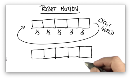
Exact Motion Quiz Solution

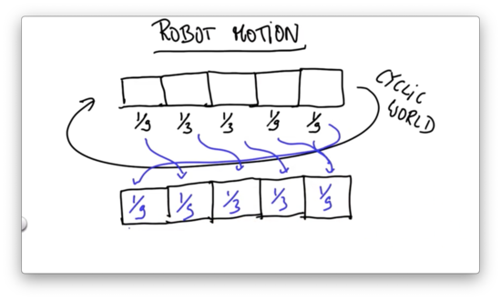
In the case of exact motion, we shift the probabilities by the direction and magnitude of the motion.

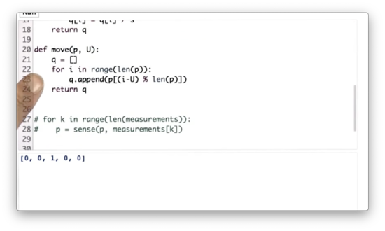
Move Function Quiz

Let's define a function, move, which takes as arguments a probability distribution, p, and a move position, U. U represents the number of places that the robot moves to the right. Our task is to implement move.

Note that our world is cyclical; that is, if a robot moves to the right of the rightmost position, it finds itself in the leftmost position.

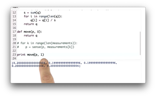
Move Function Quiz Solution

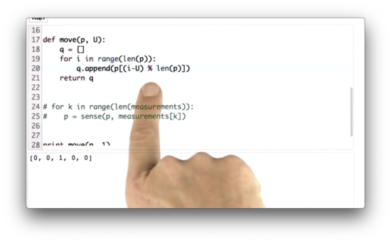
Consider a distribution, p = [0, 0.1, 0.2, 0.3, 0.4]. The resulting distribution, q, after shifting p one element to the right is [0.4, 0.1, 0.2, 0.3]. We can see that the ith element in q corresponds to the i - 1th element in p.

Of course, we need the first element in q to reference the fourth element in p. We can make our i - 1 update "wrap around" to the back of q by taking the remainder of this difference divided by len(p). Indeed, -1 % 5 = 4 in Python.

All together, given an input distribution p and a movement magnitude U, q[i] = p[i - U % len(p)], which is expressed in the code above.

Alternatively, if you are comfortable with list slicing in Python, you can just do this, as the lesson suggests:

U = U % len(p)
q = p[-U:] + p[:-U]

Inexact Motion 1 Quiz

Now let's talk about inaccurate robot motion.

We can assume that a robot executes its action correctly with high probability - 0.8 - but finds itself undershooting the target with 0.1 probability and overshooting the target with 0.1 probability.

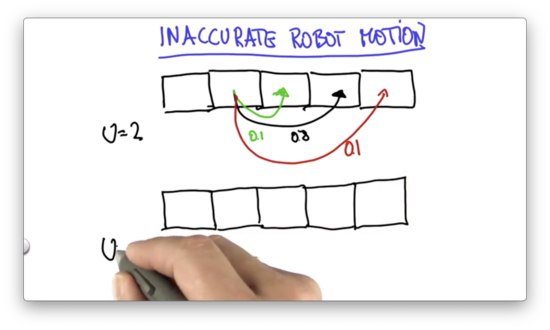
Given a motion, $U$, we can express the probabilities of undershooting, overshooting, and hitting the target position.

Given the initial probability distribution shown below, and assuming $U=2$, our task is to provide the resulting distribution after executing the inexact motion we just described.

Inexact Motion 1 Quiz Solution

Since we are sure we are starting in the second cell, we know that we end up in the third cell with probability 0.1, the fourth cell with probability 0.8, and the fifth cell with probability 0.1.

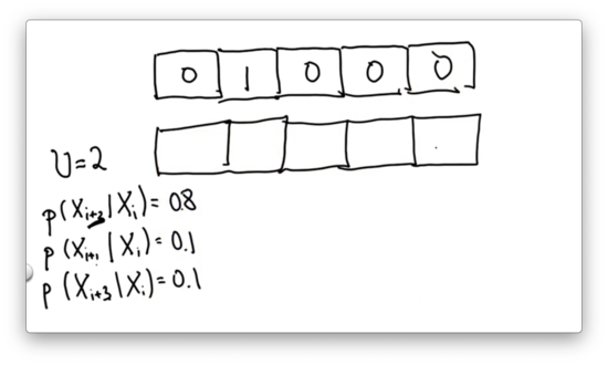
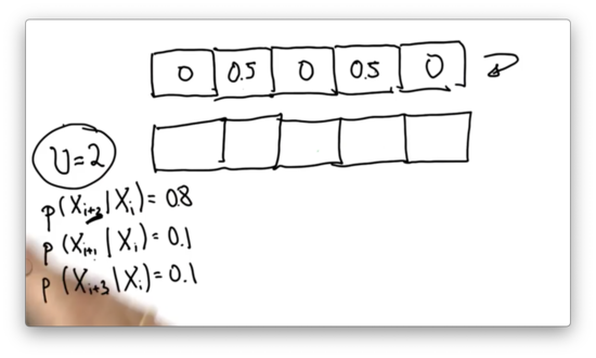
Inexact Motion 2 Quiz

Given the following input distribution, can you provide the correct posterior distribution? Assume $U=2$.

Inexact Motion 2 Quiz Solution

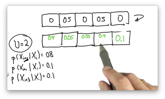
Let's look at the 0.5 associated with the second cell. Of that initial probability, 0.1 ends up in cells three and five, while 0.8 ends up in cell four. The posterior probability associated with cells three and five is 0.05, while the probability associated with cell four is 0.4.

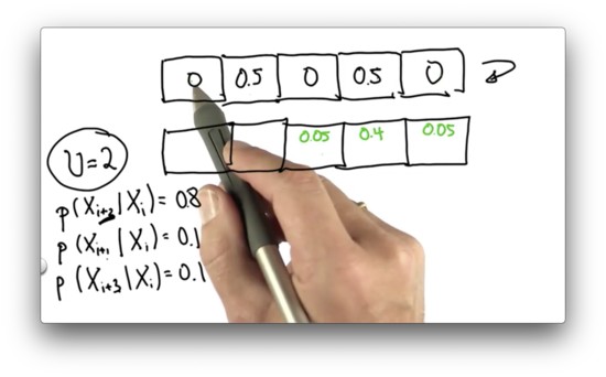
Now, let's look at the 0.5 associated with the fourth cell. Of that initial probability, 0.1 ends up in cells five and two, while 0.8 ends up in cell one. The posterior probability associated with cells five and two is 0.05, while the probability associated with cell one is 0.4.

We can see that there are two ways we might land in the fifth cell: either by overshooting from the second cell or undershooting from the fourth cell. The total probability of landing in that cell is the sum of the individual probabilities, which brings us to the final answer.

Inexact Motion 3 Quiz

Given the following uniform input distribution, can you provide the correct posterior distribution? Assume $U=2$.

Inexact Motion 3 Quiz Solution

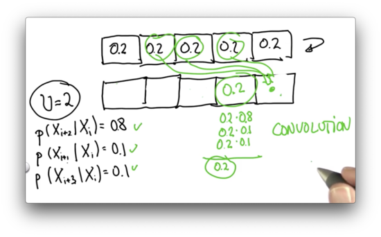
With each grid cell being equally likely in the prior distribution, each grid cell remains equally likely in the posterior distribution regardless of the uncertainty in the motion.

Let's explicitly calculate the probability of landing in the fourth cell. We could have arrived at this cell by one of three methods: overshooting from the first cell, undershooting from the third cell, or moving correctly from the second cell.

If we had a 0.2 chance of being in the first cell, and a 0.1 chance of overshooting, we have a 0.02 chance of arriving in the fourth cell by way of the first cell.

If we had a 0.2 chance of being in the second cell, and a 0.8 chance of moving correctly, we have a 0.16 chance of arriving in the fourth cell by way of the second cell.

Finally, if we had a 0.2 chance of being in the third cell, and a 0.1 chance of undershooting, we have a 0.02 chance of arriving in the fourth cell by way of the third cell.

We can add up these three probabilities to see that the chance of ending up in the fourth cell is $0.02 + 0.16 + 0.02 = 0.2$. We can show this to be true for any cell in this world.

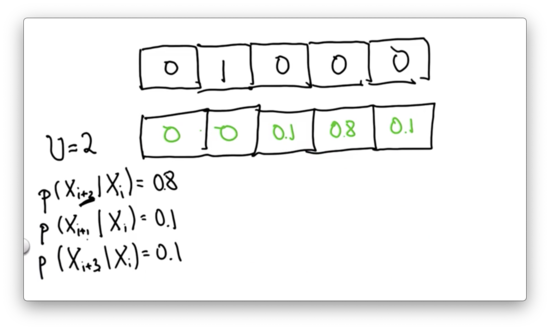
Inexact Move Function Quiz

Given three new variables, pExact = 0.8, pUndershoot = 0.1, and pOvershoot = 0.1, which represent the uncertainty in our motion, our task is to update the move function to accommodate this uncertainty.

Inexact Move Function Quiz Solution

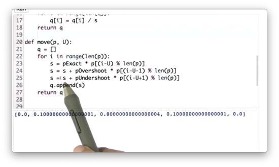
Here we introduce a temporary variable, s, which, for the ith location in the posterior distribution, represents the sum of the probabilities of reaching that location: either by undershooting from i - U + 1 places away, overshooting from i - U - 1 places away, or correctly moving from i - U places away.

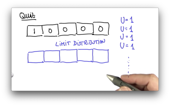
Limit Distribution Quiz

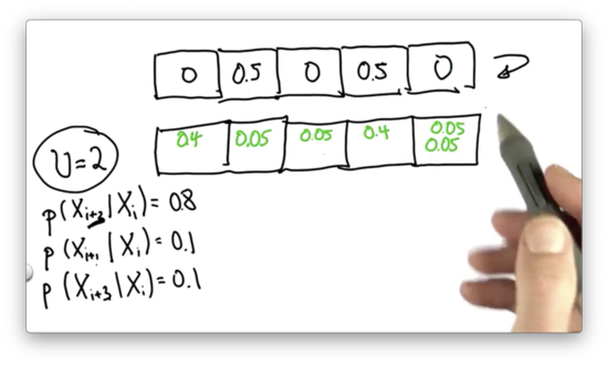
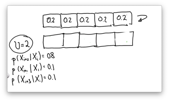
Let's assume we have the following prior distribution, and we'd like to make an inexact move one cell to the right. Assume we move correctly with probability 0.8, and we overshoot and undershoot each with probability 0.1.

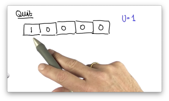
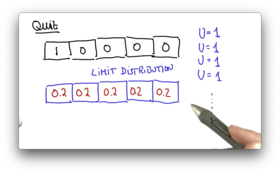
Suppose the robot runs infinitely many motion steps but never senses. What will the final posterior distribution (really, an asymptotic, or limit distribution) be after executing these motions?

Limit Distribution Quiz Quiz Solution

There is an intuitive explanation as to why our distribution converges to the uniform distribution after infinite moves.

Consider our initial distribution. We know, with certainty, that we are located in the first cell. After our motion, we can no longer say that we know where we are with certainty. There is a probability of 0.1 we are in the second or fourth cell and a probability of 0.8 we are in the second cell.

Continuing to move only serves to reduce our certainty further. We can imagine ourselves heading towards a state of maximum uncertainty: the uniform distribution.

We can think about this another way. We can consider the limit distribution as a final distribution, which doesn't change no matter how many more motions are executed. Every location in this distribution, then, must meet the following requirement:

Notice that this is the same update rule that we apply to our prior distribution based on the parameters of our motion. The only difference here is that, since we have converged, the posterior distribution calculated as a result of this update rule is always going to equal the prior distribution.

If we solve this equation, for each $X_i$ in our world, we can define the limit distribution. As it turns out, the only probability distribution where the above equation holds for all $X_i$ is the uniform distribution.

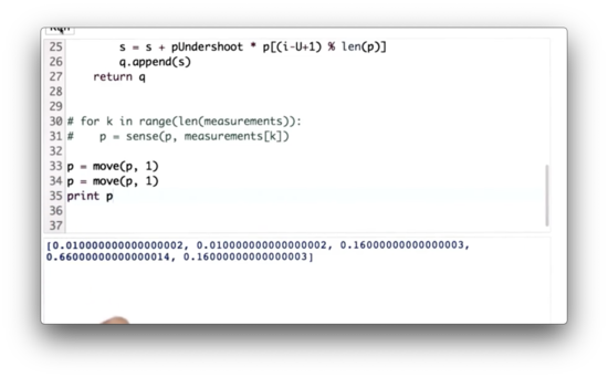
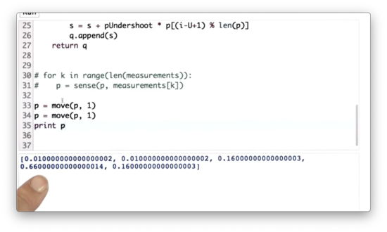
Move Twice Quiz

Let's write some code to make the robot move one space to the right two times, starting with our initial distribution, p.

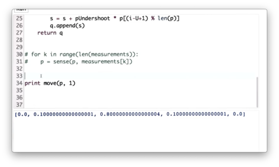
Move Twice Quiz Solution

Move 1000 Quiz

Let's write some code to make the robot move one space to the right one thousand times, starting with our initial distribution, p.

Move 1000 Quiz Solution

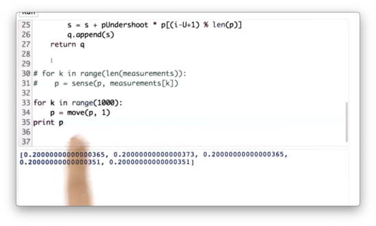
Usually, when we don't need to refer to a variable in Python, we can set it to _. For example:

for _ in range(1000):
    p = move(p, 1)

Sense and Move Quiz

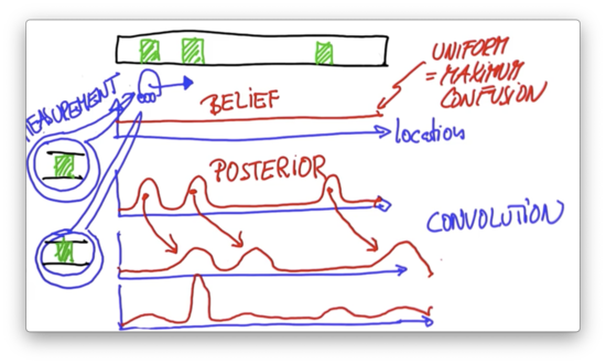
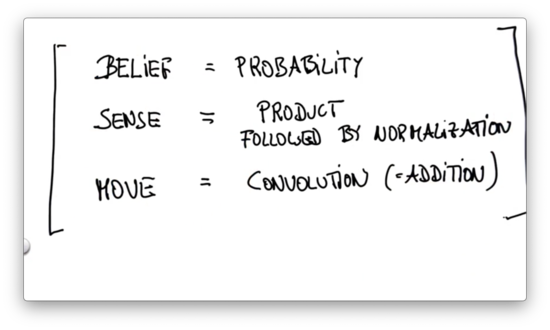
Localization is nothing more than the iteration between sense and move. We seed our localization process with an initial belief - a probability distribution - and then cycle between move and sense.

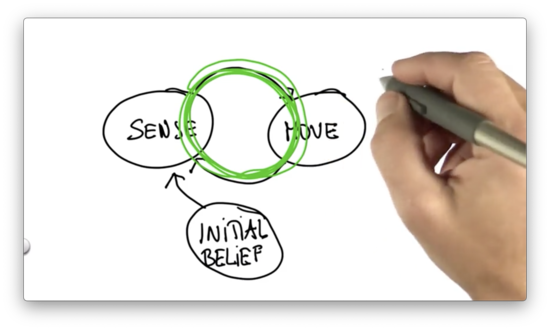
Every time the robot moves, it loses information about where it is because robot motion is inaccurate. Every time the robot senses, it gains information. This loss and gain of information are manifest by the fact that after a motion, the probability distribution is a little bit "flatter" and more "spread out", whereas after sensing its more "focused".

There is a measure of information, known as entropy, which is the expected log-likelihood of the probability of each grid cell. Without going into detail, entropy is a measure of information that the distribution has. It can be shown that the entropy increases after the motion step and decreases after the measurement step.

For more on entropy, here is the blurb from the video: Let's look at our current example where the robot could be at one of five different positions. The maximum uncertainty occurs when all positions have equal probabilities $[0.2, 0.2, 0.2, 0.2, 0.2]$.

Following the formula $Entropy = \Sigma (-p \times log(p))$, we get $-5 \times (.2)\times log(0.2) = 0.699$.

Taking a measurement will decrease uncertainty and entropy. Let's say after taking a measurement, the probabilities become $[0.05, 0.05, 0.05, 0.8, 0.05]$. Now we have a more certain guess as to where the robot is located and our entropy has decreased to 0.338.

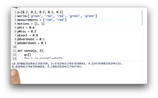
Let's assume we have a list of measurements, measurements, and a list of motions, motions. Can we use these measurements and motions, along with the sense and move functions to compute the appropriate posterior distribution?

Sense and Move Quiz Solution

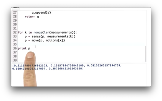
We can simply iterate through measurements and motions, sensing each measurement, and applying each motion.

Let's look at the resulting posterior distribution, p. The highest probability is associated with the fifth cell (although the corresponding probability is not 1 because our robot's motion is inexact).

This result makes sense if we look at our world, motions, and measurements.

We sensed a red cell, moved one cell to the right, sensed a green cell, and moved one cell to the right again. The most probable way for this sequence of measurements and motions to occur is by starting in the third cell, which means that we end up in the fifth cell.

Sense and Move 2 Quiz

Let's update measurements so that the robot senses "red" twice. Now which cell in the posterior distribution has the highest probability?

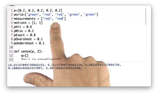
Sense and Move 2 Quiz Solution

The cell associated with the highest probability is the fourth cell. Again, this makes sense. The best match for two subsequent "red" measurements is the first "red" cell, which is the second cell overall. After two right movements, we end up in the fourth cell.

Localization Summary

We learned that localization maintains a function over all possible locations in a world, and each cell or position in that world has an associated probability value.

The measurement update function, sense, is nothing more than a product, in which we take an incoming probability distribution and multiply the probability of each location up or down depending on how well the location matches our measurement.

Additionally, we had to normalize the resulting probability function, as it might violate the fact that all probabilities in a probability distribution must add up to one.

The motion update function, move, was a convolution, whereby we determined the probability of landing on each location by looking at all of the possible paths to that location and summing their probabilities.

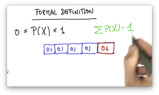
Formal Definition of Probability 1 Quiz

We can express a probability function as $P(X)$. The output of a probability function is bounded by 0 and 1; that is $0 \leq P(X) \leq 1$. $X$ often can take on multiple values, such as the five cells in our one-dimensional world.

Suppose that $X$ can only take on two values, $X_1$ and $X_2$. If $P(X_1) = 0.2$, what is $P(X_2)$?

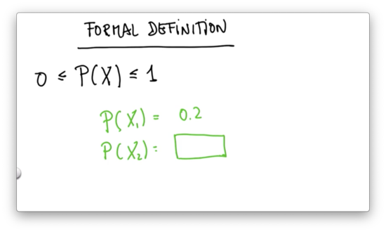
Formal Definition of Probability 1 Quiz Solution

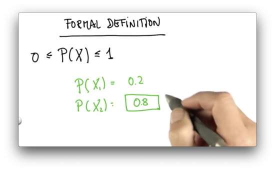
Since $P(X_1) + P(X_2) = 1$, $P(X_2) = 0.8$.

Formal Definition of Probability 2 Quiz

If $P(X_1) = 0$, what is $P(X_2)$?

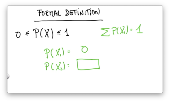
Formal Definition of Probability 2 Quiz Solution

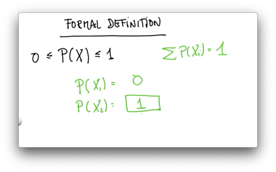
Formal Definition of Probability 3 Quiz

For our world with five grid cells, assume that $P(X_1) = P(X_2) = P(X_3) = P(X_4) = 0.1$. What is $P(X_5)$?

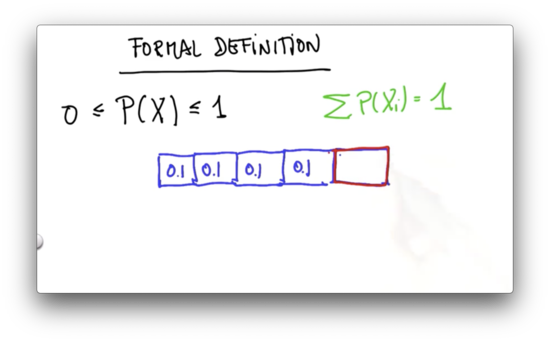
Formal Definition of Probability 3 Quiz Solution

Bayes' Rule

Suppose we have a prior distribution, $P(X)$, representing our current belief about our in the world. When we take a measurement, $Z$, we want to update $P(X)$ per $Z$.

Formally, this measurement update creates a new probability distribution that provides the probability that we are in a location, $X$, given that we took measurement $Z$. This new distribution is known as a conditional probability distribution, which we write as $P(X \mid Z)$.

Remember how we performed the measurement update. We had a prior distribution, p, along with a measurement, Z. We computed our non-normalized posterior distribution by iterating through all the probabilities in p, and multiplying each one by pHit or pMiss depending on whether the corresponding index in world matched our measurement.

Technically, pHit and pMiss are themselves conditional probabilities. When we talk about pHit, we are talking about the probability of sensing correctly; that is, the probability of taking measurement $Z$, given that the value of the current cell is $Z$. Similarly, pMiss conveys the probability of sensing incorrectly; that is, the probability of taking measurement $Z$, given that the value of the current cell is not $Z$.

What's interesting about this is that we can compute another conditional probability, $P(Z\mid X)$, which captures the probability of taking measurement, $Z$, given that we are in location $X$.

This probability takes on one of two values: either it is the probability that we measured correctly, if $Z$ is equal to the value associated with $X$, or it is the probability that we measured incorrectly if $Z$ is unequal to the value associated with $X$.

In other words, $P(Z\mid X)$ equals pHit if Z == world[i] and pMiss if Z != world[i], which is exactly what we implemented in our sense function.

To complete the calculation of our non-normalized posterior distribution, $\bar{p}(X)$, we have to multiply the probability of making the measurement $Z$ given the value of the location $X$, - $P(Z \mid X)$ - by our initial belief about our location, $P(X)$.

Recall that the sum of the probabilities in our non-normalized posterior distribution does not equal one. We can make this distribution valid by normalizing it, which we implemented in code by dividing each of the values in the posterior distribution by their sum.

We know that each value in our posterior distribution is proportional to the probability of seeing measurement $Z$ given the value at location $X$. When we add up all the individual probabilities, we can think of the resulting value as the total probability of seeing measurement $Z$, regardless of $X$.

Indeed, our normalizer, $\alpha$, is simply:

In summary, the normalized posterior distribution, $P(X \mid Z)$ is as follows:

The equation above is the equation for Bayes' rule.

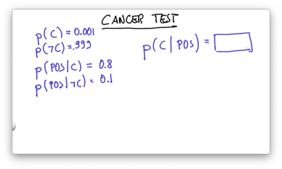
Cancer Test Quiz

Let's look at Bayes' rule in the context of cancer testing.

Suppose that there exists a certain type of cancer, the incidence of which in the population is rare. That is, $P(C) = 0.001$ and $P(\neg{C}) = 0.999$.

Furthermore, suppose we have a test which tells me I have cancer if I have cancer with probability 0.8 and tells me I have cancer if I don't have cancer with probability 0.1. That is, $P(POS \mid C) = 0.8$, and $P(POS \mid \neg{C}) = 0.1$.

What is the probability that I have cancer, given that I have received a positive test result? In other words, what is $P(C \mid POS)$?

Cancer Test Quiz Solution

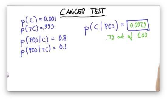
Let's remember Bayes' rule in the context of this question:

Let's first compute the non-normalized probabilities, $P(C \mid POS)$ and $P(\neg C \mid POS)$:

Note that these probabilities do not add up to one. We have to normalize them, which we can do by dividing each by their sum, which is equivalent to $P(POS)$.

As a result:

Theorem of Total Probability

Let's now look at robot motion. We are going to consider the probability of landing in cell, $X_i$, at time, $t$: $P(X_i^t)$.

Remember how we calculated this in our move function. Given $X_i$, we iterated over all cells from which we could have originated. For each origin cell, $X_j$, we took the product of the probability that we were occupying that cell and the probability that moving from that cell placed us in $X_i$ (according to the probability distribution that parameterized our inexact motion). The updated value of $X_i$ was the sum of these products.

In other words, given $j$ candidate origin cells,

The theorem of total probability states this equation in more generic terms:

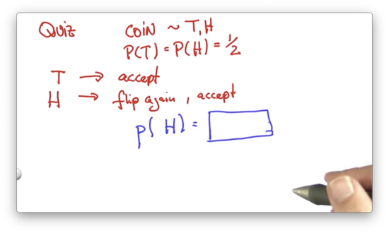
Coin Flip Quiz

Suppose we have a fair coin, which can come up either heads or tails with probability 0.5. In other words, $P(T) = P(H) = 0.5$. We flip the coin. If it comes up tails, we stop. If it comes up heads, we flip it again and stop.

What is the probability that the final result is heads?

Coin Flip Quiz Quiz Solution

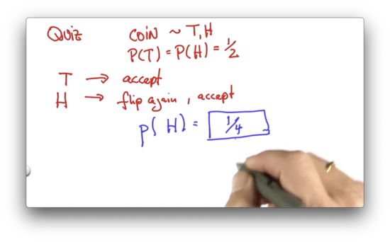
The probability of heads in step 2 is equal to the sum of two products: the probability of heads in step 2 given heads in step one times the probability of heads in step one, and; the probability of heads in step 2 given tails in step one times the probability of tails in step one.

Since we don't flip again if we see tails in step one, $P(H^2 \mid T^1) = 0$, and thus:

We know that $P(H^1) = 0.5$, since the coin is fair, and $P(H^2 \mid H^1) = P(H^2) = 0.5$ since coin flips are independent. As a result:

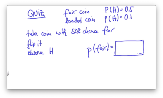
Two Coin Quiz

Let's consider two coins: a fair coin with a probability of heads, $P(H) = 0.5$, and a loaded coin with a probability of heads, $P(H) = 0.1$.

If we grab a random coin with probability 0.5, flip it, and observe heads, what is the probability that the coin we are holding is fair?

Two Coin Quiz Quiz Solution

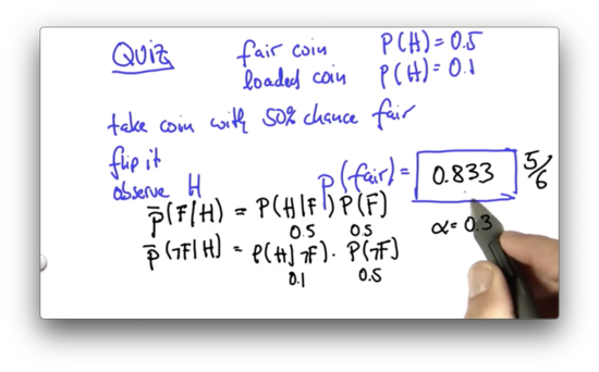
The probability that we are looking for is the probability of a fair coin, given the observation of heads: $P(F \mid H)$. We can obtain the non-normalized probability, $\bar{p}(F \mid H)$, as follows:

We know that we have a 50% chance of getting heads if we choose the fair coin, as well as a 50% chance of selecting the fair coin, so $\bar{p}(F \mid H) = 0.5 \times 0.5 = 0.25$.

We can obtain the non-normalized probability, $\bar{p}(\neg{F} \mid H)$, as follows:

We know that we have a 10% chance of getting heads if we choose the loaded coin, as well as a 50% chance of selecting the loaded coin, so $\bar{p}(\neg{F} \mid H) = 0.1 \times 0.5 = 0.5$.

Our normalizer is the sum of these two non-normalized probabilities: $\alpha = 0.25 + 0.05 = 0.3$. We can now solve for $P(F \mid H)$: