Particle Filters

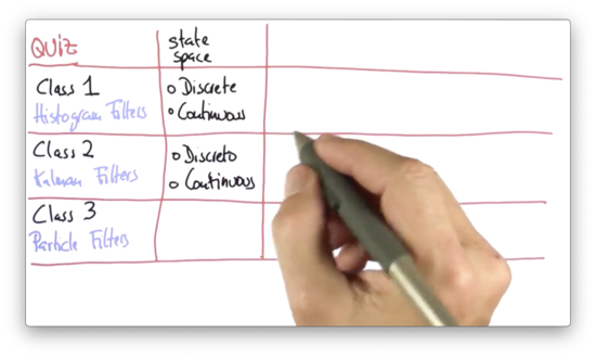
State Space Quiz

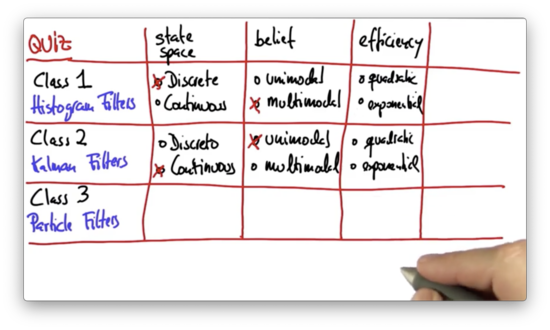
Before we start learning about particle filters, let's first review what we learned about histogram filters and Kalman filters from lessons one and two, respectively. Are histogram filters used with a continuous state space or a discrete state space? What about Kalman filters?

State Space Quiz Solution

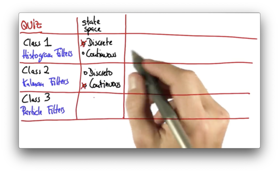
The state space for the histogram filter is discrete; that is, the distribution is defined using a finite set of bins. On the other hand, Kalman filters have a continuous state space.

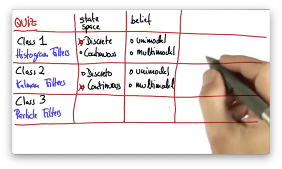
Belief Modality Quiz

Probability distributions can either be unimodal (one "peak") or multimodal (multiple "peaks"). Are the posterior distributions generated when using histogram filters multimodal or unimodal? What about the posteriors generated using Kalman filters?

Belief Modality Quiz Solution

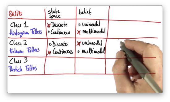
The Kalman filter is represented by a Gaussian, which, by default, is unimodal, whereas the histogram filter can have "peaks" over arbitrary grid cells.

Efficiency Quiz

From a computer memory perspective, do histogram filters scale exponentially or quadratically with regard to the number of dimensions in the measurement space? How do Kalman filters scale?

Efficiency Quiz Solution

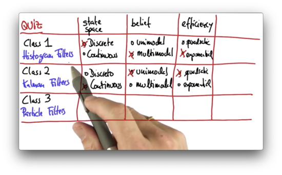
The histogram's most significant disadvantage is that it scales exponentially. Any grid that is defined over $k$ dimensions needs to represent and store $n^k$ many grid cells. For example, a two-dimensional world of five grid cells by five grid cells requires $5^2 = 25$ grid cells.

In contrast, Kalman filters grow quadratically with the number of dimensions, under certain assumptions. We represent Kalman filters with a mean vector and a covariance matrix, the latter of which is quadratic in $k$.

This scaling issue means that Kalman filters are much more efficient for problems in higher dimensions than are histogram filters and that we cannot efficiently localize in high dimensional grids using histogram filters.

Exact or Approximate Quiz

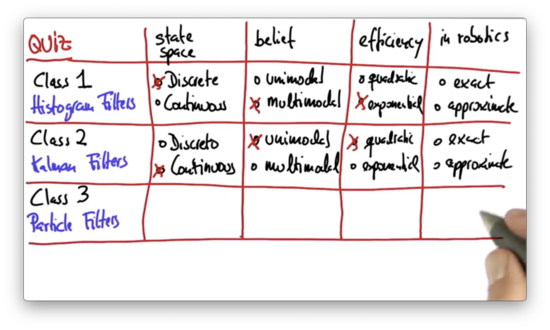
When applied to robotics, do we believe that histogram filters are exact or approximate? What about Kalman filters?

Exact or Approximate Quiz Solution

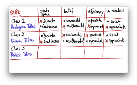
Histogram filters tend to be approximate because the world tends not to be discrete; in localization, for example, histogram filters are clearly approximate. Kalman filters are exact only for linear systems, and since the world is nonlinear, Kalman filters are effectively approximate.

Particle Filters

Like Kalman filters, the state space for particle filters is usually continuous. Similar to histogram filters, particle filters can represent arbitrary multimodal distributions. Like both filters, particle filters are approximate.

The computational complexity of particle filters is unknown. In some instances, they scale exponentially, which makes them a poor choice for state spaces with more than four dimensions. In other domains, such as tracking, they scale much more efficiently.

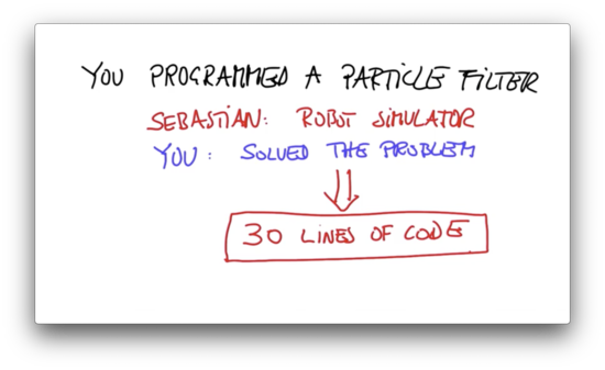
A key advantage of particle filters is that they are straightforward to program.

The animation below shows a robot performing global localization using sensor measurements. This robot has range sensors, as indicated by the blue stripes, which use sonar - sound - to determine the distance of nearby obstacles. The robot uses these range sensors to build an accurate posterior distribution of its location.

The particle filter uses particles - shown in red above - to represent the robot's best belief about its current location. In this example, each particle is represented with an x-coordinate, a y-coordinate, and a heading direction. These three values together comprise a single location estimate.

However, a single guess is not a filter. The set of several thousand such guesses - every red dot above - together comprises an approximate representation of the robot's posterior.

As the robot first begins to localize, all of the particles are uniformly spread (not shown above). The particle filter survives particles in proportion to how accurately the position of the particle aligns with the steady stream of sensor measurements.

The robot localizes itself quickly in the corridor, but two particle clouds survive because of the corridor's symmetry. As the robot enters one of the offices, however, the symmetry is broken, and the correct set of particles survives.

The essence of particle filters is to survive particles that are consistent with the measurements taken by the robot. Through this "survival of the fittest" mechanism, particles accumulate in locations that the robot is most likely to occupy. These particle clouds comprise the approximate belief of the robot as it localizes itself.

Using Robot Class

Imagine that we want to control a robot that moves about a 100-meter by 100-meter world. This robot can see four different landmarks at the following coordinates:

• 20, 20
• 80, 80
• 20, 80
• 80, 20

We can instantiate a new robot with the robot constructor:

myrobot = robot()

We can set the position of myrobot using the set method, which takes three arguments: an x-coordinate, a y-coordinate, and a heading in radians.

myrobot.set(10.0, 10.0, 0.0)

We can print myrobot.

print(myrobot)
# [x=10.0 y=10.0 heading=0.0]

We can make myrobot move with the move method. For example, we can move myrobot 10 meters forward, without turning.

myrobot = myrobot.move(0.0, 10.0)

Let's print myrobot again.

print(myrobot)
# [x=20.0 y=10.0 heading=0.0]

Let's reset myrobot, make it turn by $\frac{\pi}{2}$, and move 10 meters.

myrobot.set(10.0, 10.0, 0.0)
myrobot = myrobot.move(pi/2, 10.0)

Let's print myrobot again.

print(myrobot)
# [x=10.0 y=20.0 heading=1.5707]

We can tell myrobot to generate measurements using the sense method, which returns a list of the distances between the current position of myrobot and the four landmarks.

myrobot.sense()
# [10.0, 92.1954, 60.8276, 70.0]

Robot Class Details

The robot class defines another method, set_noise, which allows us to adjust the noisiness of moving forward, turning, and sensing.

def set_noise(self, new_f_noise, new_t_noise, new_s_noise)

Additionally, the robot class defines a method, measurement_prob, which accepts a measurement and returns the probability of such a measurement. This method is going to be very helpful in the "survival of the fittest" algorithm we are going to use to determine which particles survive and which do not.

def measurement_prob(self, measurement)

Moving Robot Quiz

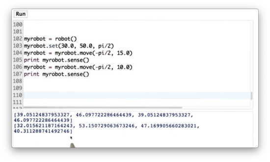
Let's take a quiz now to test out the robot class. First, set the position of myrobot to be equal to the coordinate (30, 50) with a heading of $\frac{\pi}{2}$. Next, turn myrobot clockwise by $\frac{\pi}{2}$ and move it forward 15 meters. Third, make myrobot sense and print out the measurement. Fourth, turn myrobot clockwise by $\frac{\pi}{2}$ and move it forward 10 meters. Finally, make myrobot sense again and print out the measurement.

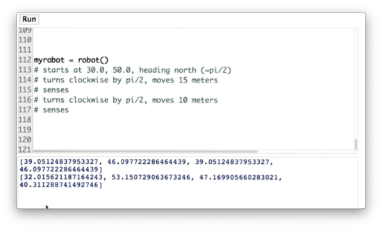
Moving Robot Quiz Solution

Add Noise Quiz

Our robot class has three built-in noise variables: one for forward movement, one for turning movement, and one for sensor measurement. We can use the set_noise method to adjust these noise variables for myrobot. Let's set the forward noise to 5.0, the turn noise to 0.1, and the sense noise to 5.0.

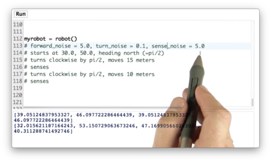
Add Noise Quiz Solution

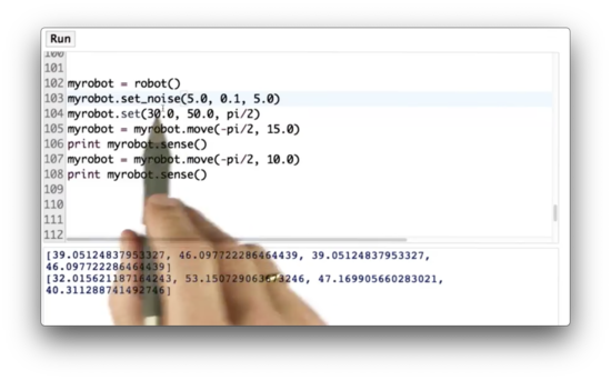
Once we introduce noise, we see that we get a different set of measurements on every run.

Robot World

Our robot can turn, move straight, and sense its distance from four different landmarks: $L_1$, $L_2$, $L_3$, and $L_4$. The robot lives in a world that is 100 meters by 100 meters, and we assume that the world is cyclical; that is, if the robot "falls off" one edge of the world, it reappears on the other edge.

Creating Particles Quiz

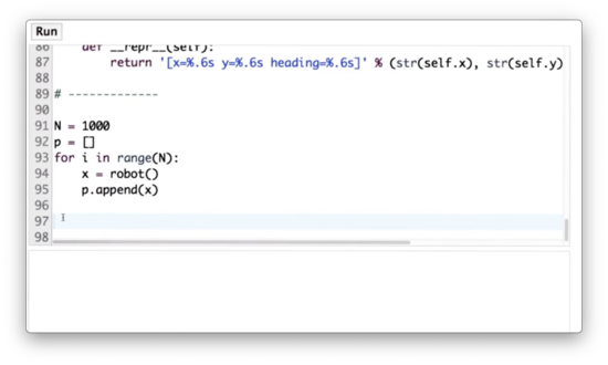
The particle filter we are going to program maintains a set of one thousand random guesses as to where the robot might be. Each guess is a vector, which contains an x-coordinate, a y-coordinate, and a heading direction.

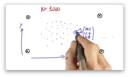
When we instantiate a new robot with the robot() constructor, the x, y, and orientation attributes are initialized at random. We can use a robot object to represent a particle. Given this information, Let's create a list of 1000 particles.

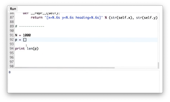
Creating Particles Quiz Solution

Robot Particles Quiz

Now let's take each of these particles and simulate robot motion. Each particle should first turn by 0.1 radians and then move forward 5 meters. Add to the code below.

Robot Particles Quiz Solution

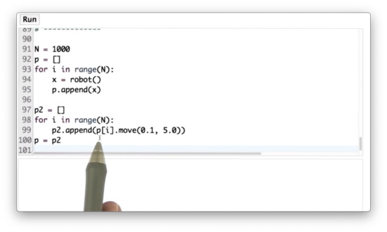
A more straightforward way to accomplish this task is shown below.

for i in range(N):
    x = robot()
    p.append(x.move(0.1, 5.0))

Importance Weight Quiz

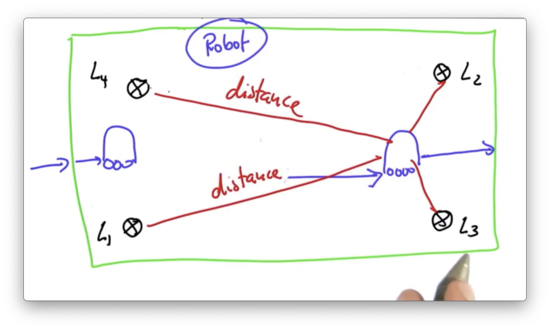
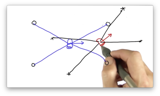
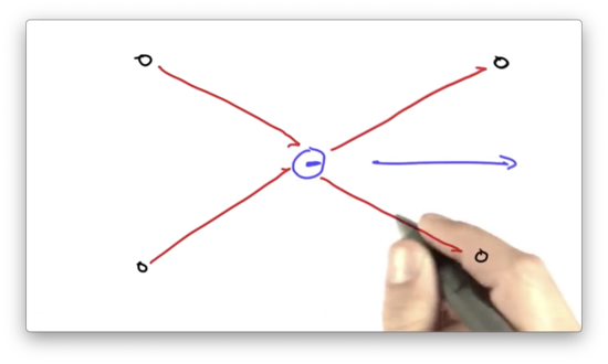
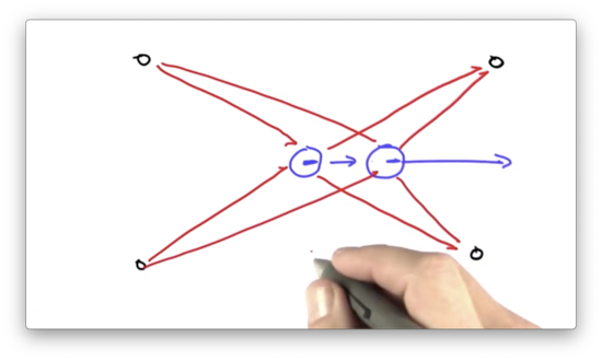
Suppose we have a robot, shown in blue below, that measures its distance from four nearby landmarks: $L_1$, $L_2$, $L_3$, and $L_4$. Consider a particle, shown in red below, that hypothesizes the robot's location and heading direction.

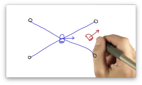
We can take the measurement vector observed by the robot and project it onto the particle.

We can see that the measurement vector, taken from the perspective of this particle, does not align with any of the landmarks in the environment. The vector we expect to see from this particle is the one drawn in green below.

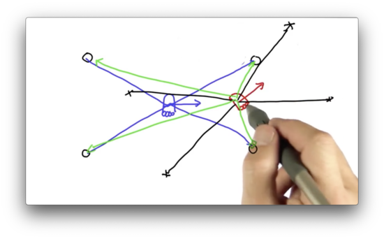
This mismatch indicates that the location of this particle is highly unlikely to coincide with the actual location of the robot. Put another way, if the robot were located at this particle, the probability of observing those particular measurements would be highly unlikely.

The difference between the actual measurement, as observed by the robot, and the predicted measurement, as observed by a particle, leads to an importance weight, which tells us how important a particular particle is. The higher the weight, the more important the particle.

When working with particle filters, we might have thousands of different particles, each with a different weight. Some particles might seem to coincide with the robot's location directly, and thus would have a more significant weight, while others might not.

During each update of the particle filter, we perform a task called resampling, whereby we randomly select $n$ new particles, with replacement, from the current pool of $n$ particles. The key is that we select new particles in proportion to their importance weight. Thus, those particles with higher importance weights are likely to live on, while those with lower weights are not likely to survive.

After a series of sensor measurements, we see particles begin to cluster around regions of a high posterior probability: the very regions where the robot is located.

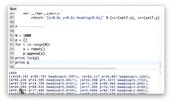
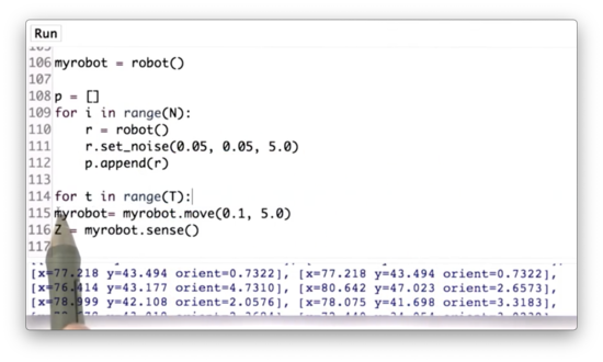
Now let's look at some code. The following code instantiates a robot, moves it a certain distance, and then reads in a sensor measurement, Z.

myrobot = robot()
myrobot = myrobot.move(0.1, 5.0)
Z = myrobot.sense()
print(Z)
# [69.5634, 15.7218, 53.1447, 47.5592]

We can also print myrobot.

print(myrobot)
# [x=33.657 y=48.869 heading=0.5567]

The robot class defines a method measurement_prob, which takes an argument measurement. The method observes its own measurement vector, dist and then returns the likelihood of observing measurement given a Gaussian centered around dist.

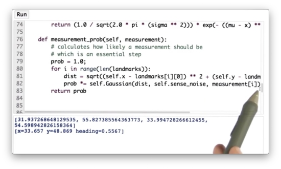
There is one additional step we need to take for this measurement probability calculation to work correctly. We need to add some measurement noise, otherwise measurement_prob ends up performing division by 0.

For a particle, x, we can set the measurement noise with the set_noise method, which takes in three arguments: one for turning noise, one for forward movement noise, and one for sensor noise.

x.set_noise(0.05, 0.05, 5.0)

Let's assume we have a list of 1000 particles, p. Our task is to create a list of 1000 importance weights, w, where w[i] contains the importance weight of the particle at p[i], given the measurement Z.

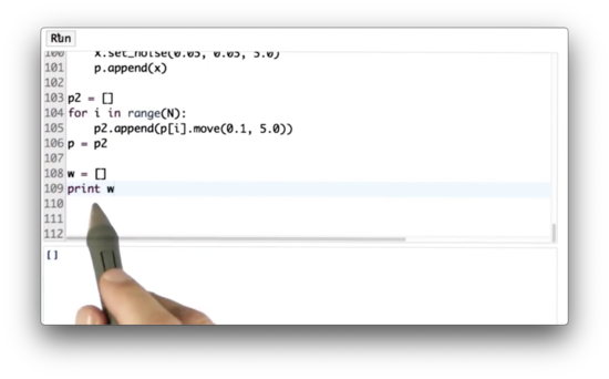
Importance Weight Quiz Solution

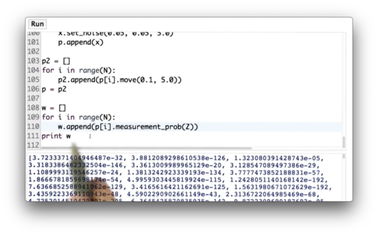
If we look at the list of weights, w, we see many minuscule probabilities, as low as $10^{-192}$, and some much larger probabilities, as high as $10^{-5}$.

In the final step of the particle filter update, we need to resample particles from p, where the likelihood of resampling any particle, p[i], is proportional to its weight, w[i].

Resampling Quiz

We are given $N$ particles, $p_1$ through $p_n$, each of which has 3 values: an x-coordinate, a y-coordinate and a heading direction. We also have $N$ weights, $w_1$ through $w_n$, each of which are floats. Let's define $W = \sum_i{w_i}$. We can use $W$ to create $N$ normalized weights, $\alpha_1$ through $\alpha_n$, where $\alpha_i = \frac{w_i}{W}$.

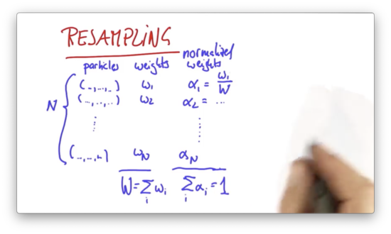
To understand resampling, imagine that all $N$ particles are placed in a bag. During the resampling process, we draw, with replacement, $N$ new particles from this bag. Each particle, $p_i$, has a probability $\alpha_i$ of being selected, which is proportional to its importance weight, $w_i$. Those particles that have a high $\alpha_i$ are likely to occur more frequently in the new set of particles.

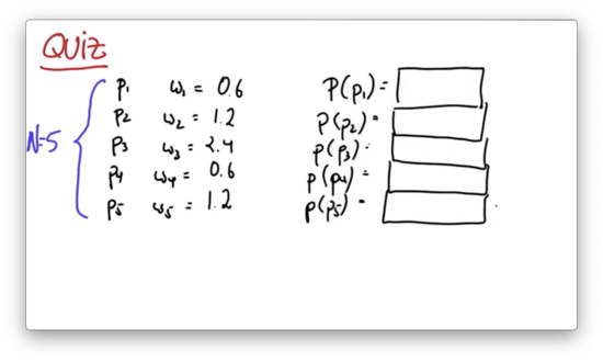
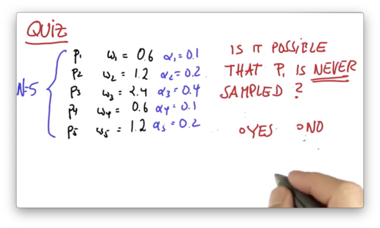
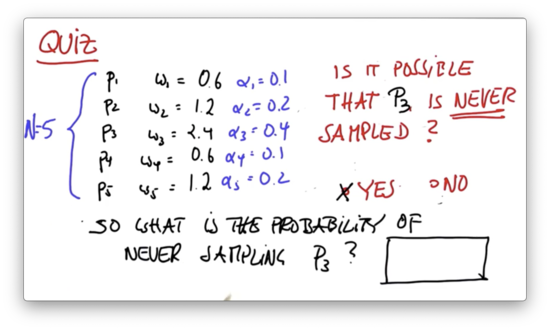
Let's test our understanding with a quiz. Given the following five particles, and the corresponding importance weights, what is the probability of drawing each particle during the resampling phase?

Resampling Quiz Solution

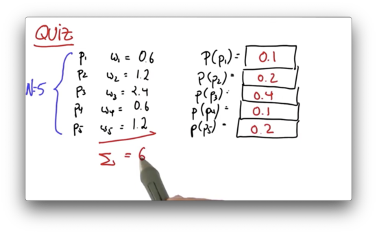
We simply add up all of the weights to get $W$, and then divide each weight, $w_i$, by $W$ to get $\alpha_i$.

Never Sampled 1 Quiz

Is it possible that $p_1$ is never sampled in the resampling step?

Never Sampled 1 Quiz Solution

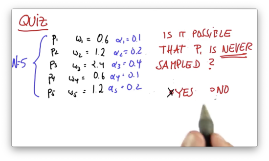
Unless a particle has an $\alpha$ of 1, it is possible for that particle not to be drawn during the resampling step.

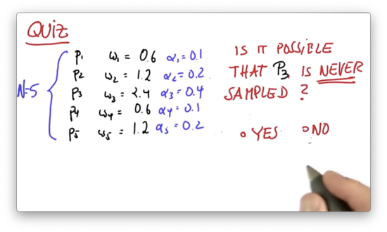
Never Sampled 2 Quiz

Is it possible that $p_3$ is never sampled in the resampling step?

Never Sampled 2 Quiz Solution

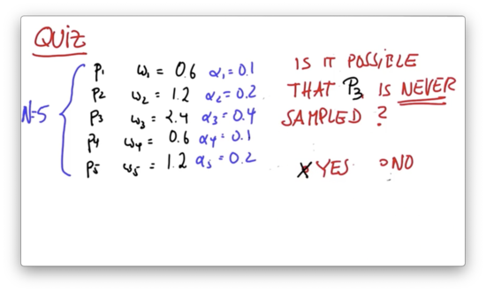
Unless a particle has an $\alpha$ of 1, it is possible for that particle not to be drawn during the resampling step.

Never Sampled 3 Quiz

Assume we make a new particle set with $N=5$ particles, where particles are drawn independently and with replacement. What is the probability of never sampling $p_3$?

Never Sampled 3 Quiz Solution

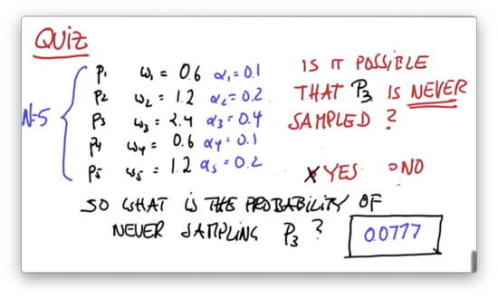
The probability of drawing $p_3$ during any round of resampling is 0.4, which means that the probability of not drawing $p_3$ is $1 - 0.4 = 0.6$. To compute the probability of not drawing $p_3$ over five independent samplings, we raise this probability to the fifth power: $0.6^5 \approx 0.0777$.

Said another way, we have an almost 93% chance of drawing $p_3$ at least once during resampling. In contrast, the probability of drawing $p_1$ at least once during resampling is $1 - 0.9^5 \approx 0.41$, or 41%.

Particles with smaller importance weights survive with a much lower probability than particles with larger importance weights, which is, of course, what we wish to achieve from the resampling step.

New Particle Quiz

Let's implement resampling now in code. Given a list of particles, p, and importance weights, w, create a new list that resamples particles from p according to the corresponding weights in w.

New Particle Quiz Solution

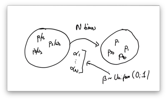
Implementing resampling is not an easy task. Here's how we might do it. First, we generate a list of all of the $\alpha$ values, alpha, from the list of weights, w, and then we sort alpha.

Next, we iterate $N$ times. For each iteration, we draw a uniform random variable, beta, in the range $[0, 1]$. We select an element, a, from alpha such that all of the values up to and including a sum to just less than beta. We then add the particle whose normalized weight is a to the list of new particles.

The runtime complexity of such a resampling procedure is $O(N\log(N))$ since sorting takes $O(N\log(N))$ time, which is not particularly efficient.

Resampling Wheel Quiz

Instead of the procedure above, we can use a more efficient algorithm that empirically gives better samples.

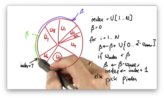
Let's represent all of the particles and their importance weights in a big wheel. Each particle occupies a slice of the wheel, where the size of the slice is proportional to the particle's importance weight.

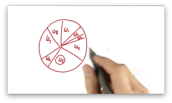
Particles that have a larger importance weight, like $w_5$, occupy more space on the wheel, whereas particles with a smaller importance weight, like $w_3$, occupy less space.

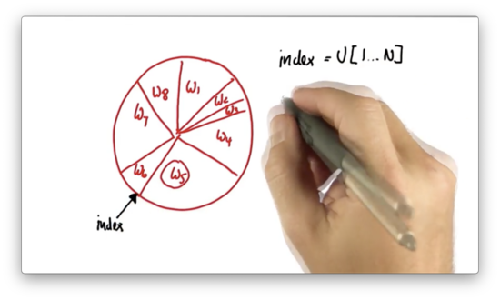
To start the resampling process, we initially draw a random number uniformly from the set of all possible particle indices: $\{0,1,2 \dots N - 1\}$. For example, if we have five particles, we will draw a number at random from the set $S = 0,1,2,3,4$.

Assume we pick the index corresponding to $w_6$, $i=5$.

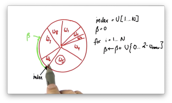
We now construct a variable $\beta$, which we initialize to $0$. We then iterate $N$ times. For each iteration, we add to $\beta$ a uniformly-drawn, continuous value that sits between $0$ and $W_{max} * 2$, where $W_{max}$ is equal to the largest importance weight. In this case, $W_{max}$ corresponds to $w_5$.

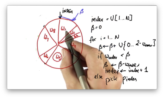
Suppose the new value of $\beta$, when added to $i$, puts us at the following location on the wheel.

Notice how $i + \beta$ corresponds to a location in the middle of the slice allocated to $w_7$. In this case - that is, when the current slice is not large enough to encapsulate $\beta$ - we subtract the weight, $w_i$, of the slice at $i$ from $\beta$ and increment $i$ by one.

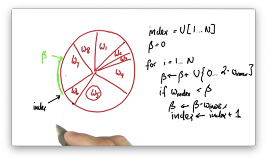
Now, $i=7$, and $w_7$ is greater than $\beta$. In this case, we pick the current particle, $p_7$, to be part of the new particle set.

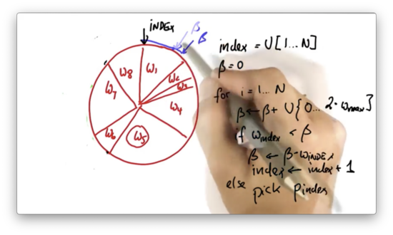
Then we repeat the process. We generate a new value of $\beta$, which is the old value plus a uniformly-drawn, continuous value that sits between $0$ and $W_{max} * 2$.

We adjust the index until it sits in the same slice as $\beta$.

Note that it is possible to randomly choose a value of $\beta$ that is small enough such that the same particle is picked twice.

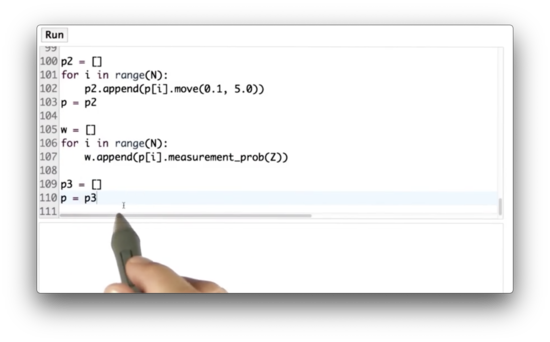
Let's implement this resampling algorithm in Python.

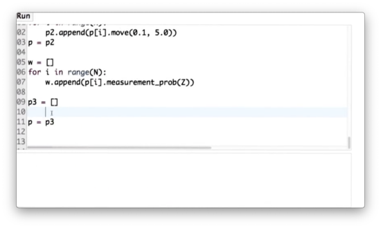
Resampling Wheel Quiz Solution

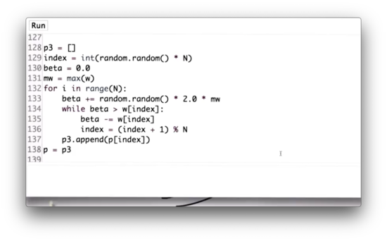
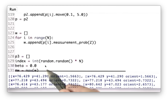
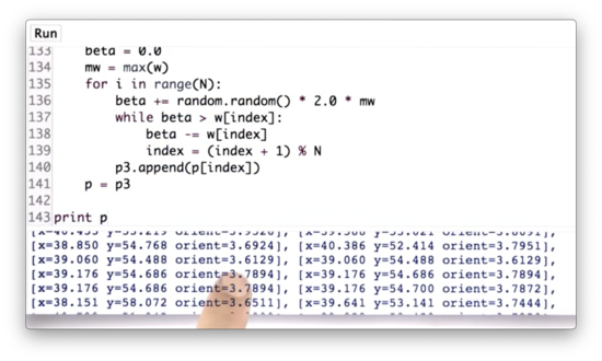
First, we create an empty list, p3, which will hold our resampled set of particles. Next, we initialize our random index, index, to an integer between 0 and N using random.random to generate a random number between 0 and 1, multiplying it by N and then casting it to an integer with int. Third, we initialize beta to 0.0 and set mw equal to the max of w.

We then iterate N times. During each iteration, we add to beta a real value drawn from a uniform random distribution over 0 to 2.0 * mw.

Next, we enter the nested iteration. While beta is larger than the weight at index, w[index], we subtract w[index] from beta and increment index by 1. Note that we wrap index around once we reach the end of w using the % operator.

Once beta <= w[index], we can append the particle at p[index] to p3. Finally, we set p = p3.

If we run this resampling step and print out p3, we can see that x and y location of the particles are very similar; in other words, the particles appear to be colocated.

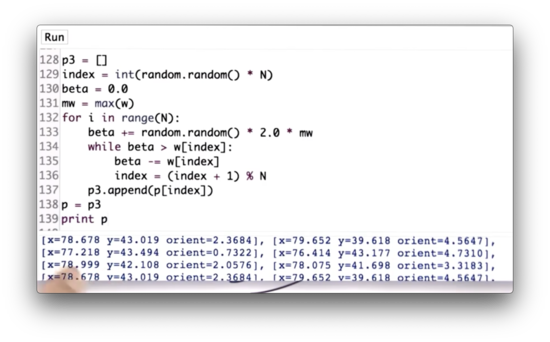
However, the orientations are not very similar. This discrepancy makes sense, given that our resampling step occurs after only one measurement. Without multiple measurements, we have no understanding of trajectory, which means we cannot estimate the robot's heading. Therefore, a particle's heading does not impact its chance of survival during this first resampling.

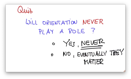
Orientation 1 Quiz

Will orientation never play a role in the resampling process?

Orientation 1 Quiz Solution

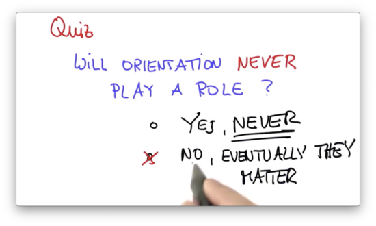
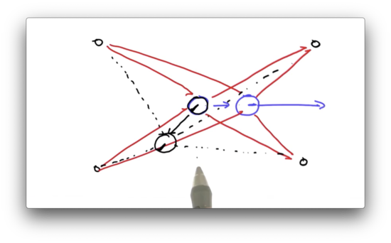
Assume we have a robot, which is facing to the right, that is positioned between four landmarks. The robot observes a set of distances between itself and the landmarks.

Now suppose the robot moves, and we observe a new set of distances.

At this point, orientation matters. If we have a particle that assumes a different initial orientation, and that particle moves, it will observe a very different set of distances. This difference will impact its chance of survival during the resampling phase, even if the particle assumed an initial position very close to the robot.

Orientation 2 Quiz

Let's update the particle filter to run twice.

Orientation 2 Quiz Solution

We can wrap the movement, sensing, and resampling steps in a for loop that iterates T times. Below are the particles after T=10 iterations, which we can see have very similar orientations.

Error Quiz

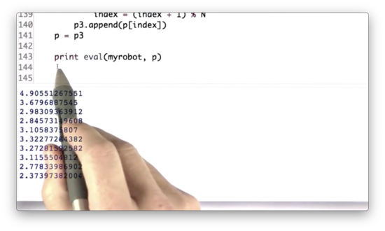
Rather than printing out the list of particles, p, let's instead print out an evaluation of our resampling step. To do this, we can use the eval function, which receives a robot, r, and a list of particles, p, and computes the average error between the particles' coordinates and the robot's coordinates.

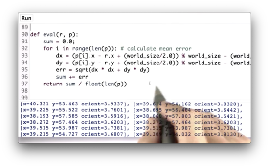
Error Quiz Solution

You and Sebastian

Filters Quiz

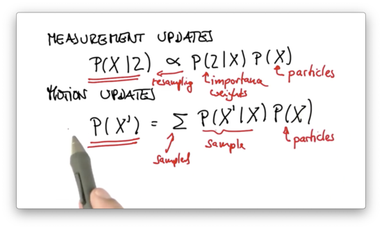
In the measurement update, we computed a posterior distribution over a state measurement, which was proportional to the probability of the measurement given the state, multiplied by the prior distribution.

In this equation, the distribution $P(X)$ is the set of particles, and the probability of the measurement given the prior, $P(Z \mid X)$, is the importance weights that correspond to those particles.

Technically speaking, $P(Z \mid X)$ is a posterior distribution. However, we wanted a posterior that didn't explicitly incorporate importance weights. By resampling, we generated the correct posterior distribution of particles according to the importance weights without having to retain those weights.

In the motion update, we computed a posterior distribution one time step later, which is the convolution of the transition probability times the prior:

As previously stated, the distribution $P(X)$ is the set of particles. We sampled from the sum by taking a random particle from $P(X)$ and applying the motion model with a noise model to generate a random particle $X^{\prime}$. As a result of this sampling, we see a new particle set, $P(X^{\prime})$, that represents the correct posterior after robot motion.

This same math underlies the histogram filters and Kalman filters we discussed in previous lessons.

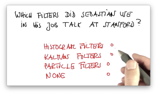
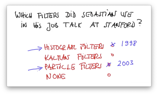
Which of the three filters did Sebastian use in his job talk at Stanford?

Filters Quiz Solution

2012

Now let's fast-forward to 2012 and the development of the Google self-driving car, which uses both histogram methods and particle methods. There are two primary differences between the implementation of the self-driving car and our current study of particle filters.

One main difference is in the robot model. The self-driving car is modeled as a system with two non-steerable wheels and two steerable wheels, often referred to as the bicycle model. This model contrasts with our (x, y, heading) representation.

The second main difference is in the sensor data. Instead of using landmarks, the self-driving car maintains an elaborate roadmap. The car periodically takes snapshots of the world and matches itself into the map from the snapshot. The better the match, the higher the score. Additionally, the self-driving car has more sensors than we discussed here, namely, GPS and inertial sensors.