Computer Networks Old
Rate Limiting & Traffic Shaping
14 minute read
Notice a tyop typo? Please submit an issue or open a PR.
Rate Limiting & Traffic Shaping
Traffic Classification and Shaping
This lesson focuses on ways to classify traffic as well as several traffic shaping strategies, including
- leaky bucket
- (r, T) traffic shaper
- token bucket
- composite traffic shaper
The motivation behind traffic shaping is to control traffic resources and ensure that no traffic flow exceeds a particular pre-specified rate.
Source Classification
Traffic sources can be classified in many different ways.
Data traffic may be bursty, and may be periodic or regular. Audio traffic is usually continuous and strongly periodic. Video traffic is continuous, but often bursty due to the nature of how video is often compressed.
We usually classify traffic sources according to two kinds of traffic.
One is constant bit rate (CBR) source. In a constant bit rate traffic source, traffic arrives at regular intervals, and packets are typically the same size, resulting in a constant bit rate of arrival. Audio is an example of a constant bit rate source.
Many other sources of traffic are variable bit rate (VBR). Video and data traffic are often variable bit rate.
When we shape CBR traffic, we tend to shape according to the peak rate. VBR traffic is often shaped according to an average rate and a peak rate.
Leaky Bucket Traffic Shaping
In a leaky bucket traffic shaper, traffic arrives in a bucket of size and drains from the bucket at rate . Each traffic flow has its own bucket.
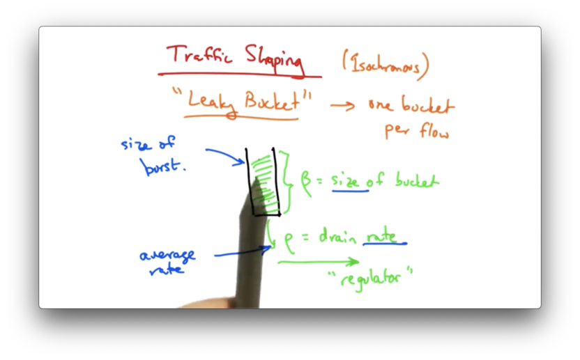
While traffic can flow into the bucket at any rate, it cannot drain from the bucket at a rate faster than . Therefore, the maximum average rate that data can be sent through this bucket is .
The size of the bucket controls the maximum burst size that a sender can send for a particular flow. Even though the average rate cannot exceed , the sender may be able to, at times, send at a faster rate, as long as the total size of the burst does not overflow the bucket.
Setting a larger bucket size can accommodate a larger burst rate. Setting a larger value of can enable a faster packet rate.
In short, the leaky bucket allows flows to periodically burst while maintaining a constant drain rate.
Audio Example
For an audio application, one might consider setting the size of the bucket to 16kB, so packets of 1kB would then be able to accumulate a burst of up to 16 packets into the bucket.
The regulator's rate of 8 packets per second, however, would ensure that the audio rate would be smooth to an average rate not to exceed 8kB / second, or 64kbps.
(r, T) Traffic Shaping
In (r, T) traffic shaping traffic is divided in T-bit frames, and a flow can inject up to r bits in any T-bit frame.
If the sender wants to send more than one packet of r bits, it simply has to wait until the next T-bit frame.
A flow that obeys this rule has an (r, T) smooth traffic shape.
In (r, T) traffic shaping a sender can't send a packet that is larger than r bits long. Unless T is very large, the maximum packet size may be very small, so this type of traffic shaping is typically limited to fixed-rate flows.
Variable flows have to request data rates that are equal to the peak rate. It would be incredibly wasteful to configure the shaper such that the average rate must support whatever peak rate the variable rate flow must send.
The (r, T) traffic shaper is slightly relaxed from a simple leaky bucket. Rather than sending one packet per every time unit, the flow can send a certain number of bits every time unit.
If a flow exceeds a particular rate, the excess packets in the flow are typically given a lower priority. If the network is heavily congested, the packets from a flow that exceeds its rate may be preferentially dropped.
Priorities might be assigned at the sender or at the network.
At the sender, the application might mark its own packets, since the application knows best which packets may be more important. In the network, the routers may mark packets with a lower priority, a feature known as policing.
Shaping Bursty Traffic Patterns
Sometimes we want to shape bursty traffic, allowing for bursts to be sent on the network, while still ensuring that the flow doesn't exceed some average rate.
For this scenario, we might use a token bucket.
In a token bucket, tokens arrive in a bucket at a rate . Again, is the capacity of the bucket. Traffic may arrive at an average rate and a peak rate.
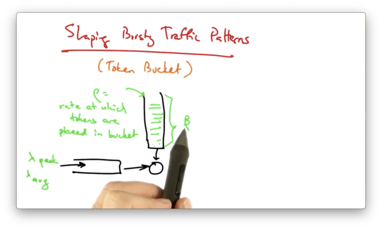
Traffic can be sent by the regulator as long as there are sufficient tokens in the bucket.
To consider the difference between a token bucket and a leaky bucket, consider sending a packet of size b < .
If the token bucket is full, the packet is sent, and b tokens are removed.
If the token bucket is empty, the packet must wait until b tokens drip into the bucket.
If the bucket is partially full, the packet may or may not be sent. If the number of tokens in the bucket exceed b, then the packet is sent immediately and b tokens are removed. Otherwise, the packet must wait until b tokens are present in the bucket.
Token Bucket vs Leaky Bucket
A token bucket permits traffic to be bursty but bounds it by the rate . A leaky bucket forces the bursty traffic to be smooth.
If our bucket size in a token bucket is , we know that for any interval T, our rate must be less than plus the rate that which tokens accumulate () times T.
Intuitively, this makes sense. We can completely drain the bucket and also consume the tokens that are added to the bucket over the interval T, which *T.
We also know that the long-term rate will always be less than .
Token buckets have no discard or priority policies, while leaky buckets typically implement priority policies for flows that exceed the smoothing rate.
Both token buckets and leaky buckets are relatively easy to implement, but the token bucket is a little bit more flexible since it has additional parameters for configuring burst size.
One of the limitations of token buckets is that in any interval of length T, the flow can send + T* tokens of data.
If a network tries to police the flows by simply measuring the flows over intervals of length T, the flow can cheat by sending + T* traffic in each interval.
Consider an interval of 2T. If the flow can send + T in each interval, the flow can send 2( + T ) in an interval of 2T, which is greater than what it should be allowed to send: + 2T * .
Policing traffic being sent by token buckets can be rather difficult.
Token buckets allow for long bursts. If the bursts are of high priority traffic, they are difficult to police and may interfere with other high priority traffic.
There is a need to limit how long a token bucket can sender can monopolize the network.
Policing With Token Buckets
To apply policing to token buckets, one strategy is to use a composite shaper, which combines a token bucket and a leaky bucket.
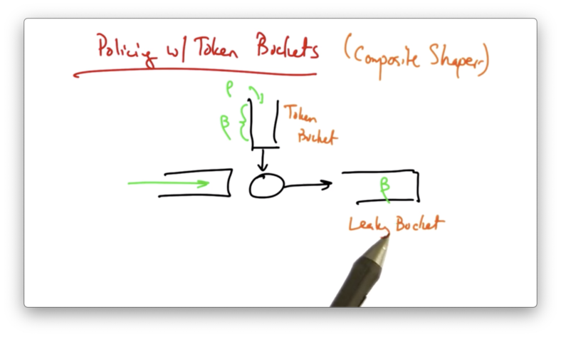
The combination of the two ensures that a flow's data rate doesn't exceed the average data rate enforced by the smooth leaky bucket.
The implementation is more complex, though, since each flow now requires two timers and two counters, one for each bucket.
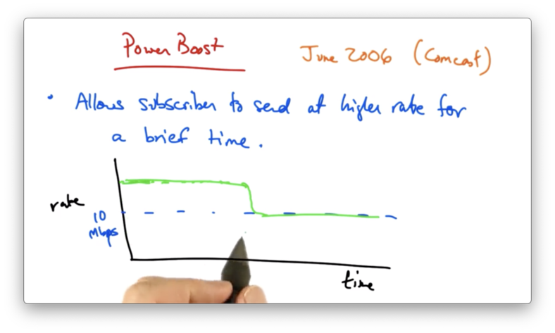
Power Boost
Power boost allows a subscriber to send at a higher rate for a brief period of time.
For example, if you subscribed at a rate of 10Mbps, power boost might allow you to send at a higher rate for some period of time before being shaped back to the rate at which you subscribed at.
Power boost targets the spare capacity in the network for use by subscribers who don't put sustained load on the network.
There are two types of power boost.
If the rate at which the user can achieve during the burst window is set to not exceed a particular rate, the power boost is capped. Otherwise, the power boost is uncapped.
In the uncapped setting, the change to the traffic shaper is simple. The size of the token bucket is increased. Since the rate of flow through a token bucket depends on , a larger bucket size will be able to sustain a bigger burst.
In this case, the maximum sustained traffic rate is remains .
If we want to cap the rate, all we need to do is simply apply a second token bucket with another value of .
That token bucket limits the peak sending rate for power boost eligible packets to , where P is larger than .
Since plays a role in how quickly tokens can refill in the bucket, so it also plays a role in the maximum rate that can be sustained in a power boost window.
Calculating Power Boost Rates
Suppose that a sender is sending at some rate R which is greater than their subscribed rate r. Suppose as well that the power boost bucket size is .
How long can a sender send at rate R?
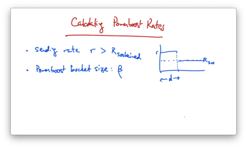
Given the diagram above, we need to solve for d.
We know that the is d * (R - r) , so if we solve for d, we see that d is equal to $\beta$ / (R - r).
Examples of Power Boost
Here is a graph (courtesy of the BISmark project) measuring the power boost experienced by four different home networks - each with a different cable modem - connecting through Comcast.
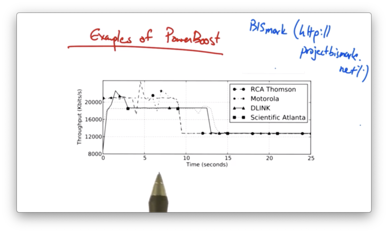
Different homes exhibit different shaping profiles: some have a very steady pattern, whereas others have a very erratic pattern.
In addition, it appears that there are two different tiers of higher throughput rates.
Effects on Latency
Even though power boost allows users to send at a higher traffic rate, users may experience high latency and loss over the duration that they are sending at this higher rate.
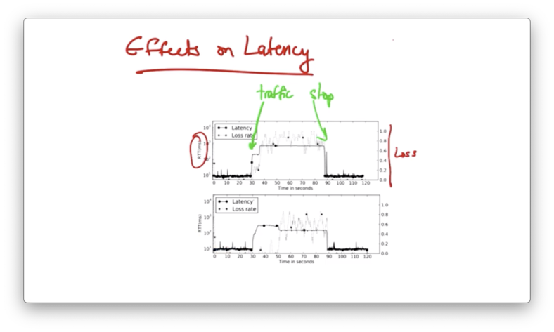
The reason for this is that the access link may not be able to support the higher rate.
If a sender can only send at some sustained rate R for an extended period of time, but is allowed to send at a boosted rate r for a short period of time, buffers may fill up.
TCP senders can continue to send at the higher rate r without seeing packet loss even though the access link may not be able to send at that higher rate.
As a result, packets buffer up and users see higher latency over the course of the power boost interval.
To solve this problem, a sender might shape its rate never to exceed the sustained rate R. If it did this, it could avoid seeing these latency effects.
Certain senders who are more interested in keep latency under control than sending at bursty volumes may choose to run such a traffic shaper in front of a power boost enabled link.
Buffer Bloat
The increase in latency as a result of power boost that we visualized in the previous section is an example of buffer bloat.
Buffer bloat occurs when a sender is allowed to send at some rate r that is greater than the sustained rate R without seeing packet loss.
A buffer in the network that can support this higher rate will start filling up with packets. Since the buffer can only drain at R, all of the packets that the sender is sending at r are just being queued up in the buffer.
As a result, the packets will see higher delay than they would if they simply arrived at the front of the queue and could be sent immediately.
The delay that a packet arriving in a buffer will see is the amount of data ahead of it in the buffer divided by the sustained rate R.
These large buffers can introduce delays that ruin the performance for time-critical applications such as voice and video applications.
These larger buffers can be found in
- home routers
- home access points
- hosts on device drivers
- switches and routers
Buffer Bloat Example
Let's look at the round trip times for 3 different DSL routers.
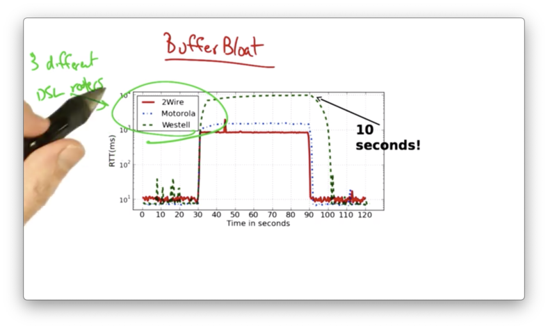
An upload was started at 30 seconds.
We can see that the modems experience a huge increase in latency coinciding with the start of the upload. The routers saw an increase in RTT up to 1 second and even 10 seconds, up from the typical RTT of 10ms.
A home modem has a packet buffer. Your ISP is upstream of that buffer, and the access link is draining that buffer at a certain rate.
TCP senders in the home will send until they see lost packets. If the buffer is large, the senders won't actually see those lost packets until this buffer has already filled up.
The senders continue to send at increasingly faster rates until they see a loss. As a result, packets arriving at this buffer see increasing delays, while senders continue to send at faster and faster rates.
There are several solutions to the buffer bloat problem.
One obvious solution is to use smaller buffers. Given that we already have a lot of deployed infrastructure, however, simply reducing the buffer size across all of that infrastructure is not a trivial task.
Another solution is to use traffic shaping. The modem buffer drains at a particular rate, which is the rate of the uplink to the ISP. If we shape traffic such that traffic coming into the access link never exceeds the uplink provided by the ISP, the buffer will never fill.
This type of shaping can be done on many OpenWRT routers.
Network Measurement
There are two types of network measurement.
In passive measurement, we collect packets and flow statistics from traffic that is already being sent on the network.
This might include
- packet traces
- flow metrics
- application logs
In active measurement, we inject additional traffic into the network to measure various characteristics of the network.
Common active measurements tools include
Ping is often used to measure the delay to a particular server, while traceroute is used to measure the network-level path between two hosts on the network.
Why Measure
Why do we want to measure traffic on the network?
Billing
We might want to charge a customer based on how much traffic they have sent on the network. In order to do so, we need to passively measure how much traffic that customer is sending.
A customer commonly pays for a committed information rate (CIR). Their network throughput will be measured every five minutes, and they will be billed on the 95th percentile of these five minute samples. This mode of billing is called 95th percentile billing.
This means that the customer might be able to occasionally burst at higher rates without incurring higher cost.
Security
Network operators may also want to know the type of traffic being sent on the network so they can detect rogue behavior.
A network operator may want to detect
- compromised hosts
- botnets
- denial of service attacks
How to Measure Passively
One way to perform passive traffic management is to use the packet and byte counters provided by the Simple Network Management Protocol (SNMP).
Many network devices provide a Management Information Base (MIB) that can be polled/queried for particular information.
One common use for SNMP is to poll a particular interface on a network device for the number of bytes/packets that is has sent.
By periodically polling, we can determine the rates at which traffic is being sent on a link, and taking the difference in the counts divided by the interval between measurements.
The advantage of SNMP is that is fairly ubiquitous: it's supported on basically all networking equipment. There are many products available for polling/analyzing SNMP data.
On the other hand, the data is fairly course. Since SNMP only allows for polling byte/packet counts on the interface, we can't ask really analyze specific hosts or flows.
Two other ways to measure passively are by monitoring at a packet-level granularity or flow-level granularity. At the packet level, monitors can see full packet contents (or at least headers). At the flow level, a monitor may see specific statistics about individual flows in the network.
Packet Monitoring
In packet monitoring, the monitor may see the full packet contents - or at least the packet headers - for packets that traverse a particular link.
Common packet monitoring tools include
Sometimes, packet monitoring is performed using expensive hardware that can be mounted in servers alongside routers that forward traffic through the network.
In these cases, an optical link in the network is sometimes split, so that traffic can be both sent along the network and sent to the monitor.
Even though packet monitoring sometimes requires expensive hardware on high speed links, the software-based packet monitoring tools essentially do the same thing.
These tools allow your machine to act as a monitor on the local area network, and if any packets are sent towards your network interface, the monitor records those packets.
On a switched network, you wouldn't see many packets that weren't destined for your MAC address, but on a network where there is a lot of traffic being flooded, you might see quite a bit more traffic destined for an interface that you are using to monitor.
The advantages of packet monitoring is that it provides lots of detail, like timing information and information gleaned from packet headers.
The disadvantage of packet monitoring is that there is relatively high overhead. It's very hard to keep up with high speed links, and often requires a separate monitoring hardware device.
Flow Monitoring
A flow consists of packets that share a common
- source/destination IP address
- source/destination port
- protocol type
- TOS byte
- interface
A flow monitor can record statistics for a flow that is defined by the group of packets that share these features.
Flow records may also contain additional information, often related to routing, such as
- next-hop IP
- source/destination AS
- prefix
Flow monitoring has less overhead than packet monitoring, but it is more coarse than packet monitoring.
Because a flow monitor can not see the individual packets, it is impossible for the monitor to surface some types of information, such as information about packet timing.
In addition to grouping packets into flows based on common data elements, packets are also typically grouped into flows if they occur close together in time.
For example, if packets that share common sets of header fields do not appear during a particular time interval - say, 15 or 30 seconds - the router simply declares the flow to be over, and sends the statistics to the monitor.
Sometimes, to reduce monitoring overhead, flow level monitoring may also be accompanied by sampling.
Sampling builds flow statistics based only on samples of the packets. For example, flows may be created based on one out of every ten or 100 packets, or a packet might be sampled with a particular probability.
Flow statistics may be based on the packets that are sampled randomly from the total set of packets.
OMSCS Notes is made with in NYC by Matt Schlenker.
Copyright © 2019-2023. All rights reserved.
privacy policy