Computer Networks Old
Traffic Engineering
14 minute read
Notice a tyop typo? Please submit an issue or open a PR.
Traffic Engineering
Traffic Engineering Overview
Traffic engineering is the process of reconfiguring the network in response to changing traffic loads in order to achieve some operational goal.
A network operator may want to reconfigure the network in order to
- maintain traffic ratios with peers
- relieve congestion on certain links
- balance load more evenly
In some sense, IP networks manage themselves. For example, TCP senders send less traffic in response to congestion and routing protocols will adapt to topology changes.
The problem is that even though these protocols are designed to adapt to various changes, the network may still not run efficiently.
For instance, there may be congested links when idle paths exists or there might be a high delay path that some packet is taking when a low delay path exists.
A key question that traffic engineering seeks to address is: How should routing adapt to traffic?
In particular, traffic engineering seeks to avoid congested links and satisfy certain application requirements, such as delay.
Intradomain Traffic Engineering
Suppose we have a single autonomous system with the following static link weights.
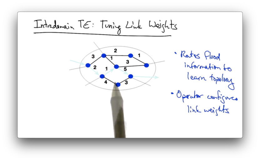
An operator can affect the shortest path between two nodes in the graph by configuring the link weights, thus affecting the way that traffic flows through network.
Suppose that the operator of this network above would like to shift traffic off of a congested link in the middle of the network.
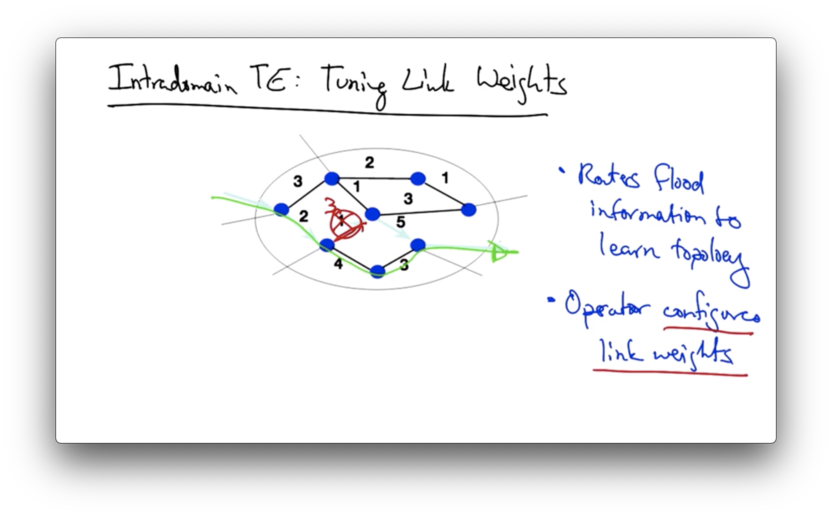
By changing the link weight from 1 to 3, the shortest path between the two nodes now takes an alternate route.
In practice, link weights can be set in a variety of ways:
- inversely proportional to capacity
- proportional to propagation delay
- according to some network-wide traffic optimization goal
Measuring, Modeling and Controlling Traffic
Traffic engineering has three main steps.
First, we must measure the network to figure out the current traffic loads. Next, we need to form a model of how configuration affects the underlying paths in the network. Finally, we reconfigure the network to exert control over how traffic flows through the network.
An operator might measure the topology and traffic of a network, feed that topology and traffic to a prediction model that estimates the effect of various types of configuration changes, decide which changes to make, and then adjust link weights accordingly.
Intradomain traffic engineering attempts to solve an optimization problem, where the input is a graph G, parameterized by nodes R - the set of routers - and edges L - the set of unidirectional links.
Each link l has a fixed capacity c_l.
Another input to the optimization problem is the traffic matrix, where M_ij represents the traffic load from router i to router j.
The output of the optimization problem is a set of link weights, where W_l is the weight on any unidirectional link l.
Ultimately, the setting of these link weights should result in a fraction of the traffic from i to j traversing each link l, for every i, j, and l such that those fractions satisfy some network-wide objective.
Link Utilization Function
The cost of congestion increases in a quadratic manner as the loads on the links continue to increase, approaching infinite cost as link utilization approaches 1.
We can define utilization as the amount of traffic on a link divided by the capacity of that link.
Solving the optimization problem is much easier if we approximate the "true" quadratic cost function (orange below) with a piecewise, linear function (blue below).

Our objective might be to minimize the sum of this piecewise linear cost function over all the links in the network.
Unfortunately, this optimization problem NP-complete, which means that there is currently no efficient algorithm to find the optimal setting of link weights even for simple objective functions.
Instead, we must iteratively search through a large set of combinations of link weights to find a good setting. While this search is suboptimal, the graphs are often small enough in practice to allow this approach to be effective.
In practice, we also have other operational realities to worry about. For example, we'd often like to limit the number of changes we make to the network and the frequency with which we make these changes.
In addition, whatever solution we come up with must be resistant to failure and it should be robust to measurement noise.
BGP in Interdomain Traffic Engineering
Interdomain routing concerns routing between autonomous systems and involves the reconfiguration of BGP policies running on individual routers in the network.
Changing BGP policies at the edge routers can cause routers inside an AS to direct traffic towards or away from certain edge links.
An operator might with wish to use interdomain traffic engineering if
- a link is congested
- a link is upgraded
- a peering agreement is violated
For example, AS 1 and AS 2 might have an agreement where they only send a certain amount of traffic to one another during a particular time window.
If AS 1 begins to exceed the limit for traffic it is allowed to send to AS 2 the operator would need to use BGP to shift traffic from that egress link to another.
Interdomain Traffic Engineering Goals
Interdomain traffic engineering has three main goals.
Predictability
It should be possible to predict how traffic flows will change in response to changes in the network configuration.
Suppose that a downstream AS D is trying to reach is trying to reach upstream neighbor U, and is currently routing traffic through neighbor AS N.
N may wish to relieve congestion on the particular link that it is using currently to forward the traffic from D to U . To so do, it might forward that traffic out a different egress, likely through a different set of ASes.
Once N makes that change, the traffic might now be taking a longer AS path and, in response, D might decide to not route traffic through N at all.
All of the work that went in to optimizing traffic load balance for N is now for naught, because the change that it made changed the traffic matrix that it now experiences.
One way to avoid this problem and achieve predictable traffic changes is to avoid making changes that are globally visible.
In particular, this change made a change in the AS path length of the advertisement from N to U.
Thus other neighbors - like D - might decide to use another path as a result of that globally visible routing change.
Limit influence of neighbors
Another goal of interdomain traffic engineering is to limit the influence of neighboring ASes.
Specifically, we'd like to use BGP policies and changes to those policies that limit how neighboring ASes might change their behavior in response to changes to the BGP configuration that we make in our own network.
For example, an AS might try to make a path look longer with AS path prepending.
If we consider treating paths that have almost the same AS path length as a common group, we can achieve additional flexibility.
Additionally, if we enforce a constraint that our neighbors should advertise consistent BGP route advertisements over multiple peering links (should multiple links exist), our network will have additional flexibility to send traffic over different egress points to the AS.
Enforcing consistent advertisements turns out to be difficult in practice.
Reduce overhead of routing changes
A third goal of interdomain traffic engineering is to reduce the overhead of routing changes; that is, we'd like to achieve our network goals with changes to as few IP prefixes as possible.
To achieve this, we can group related prefixes. Rather than exploring all combinations of prefixes in order to move a particular volume of traffic, we can identify routing choices that group routes that have the same AS paths, and we can move groups of prefixes according to the groups of prefixes that share an AS path.
We can move these groups easily by making tweaks to local preference values using regular expressions on AS path.
We can also choose to focus only on the small fraction of prefixes that carry the majority of the traffic.
Since 10% of origin ASes are responsible for about 82% of outbound traffic, we can achieve significant gains by focusing primarily on traffic destined for these ASes.
Multipath Routing
Another way to perform traffic engineering is with multipath routing, whereby an operator can establish multiple paths in advance.
This approach can be applied to both interdomain and intradomain routing.
In intradomain routing, we can achieve this by setting link weights such that multiple paths of equal cost exist between multiple nodes in the graph, an approach called equal cost multipath (ECMP).
As a result of ECMP, traffic will be split across paths that have equal cost in the network.
A source router might also be able to change the fraction along each one of these paths, sending for example 35% along one path and 65% along the other.
To achieve this, the router would multiple forwarding table entries with different next hops for outgoing packets to the same destination.
Data Center Networking
Data center networks have three main characteristics:
- multi-tenancy
- elastic resources
- flexible service management
Multi-tenancy allows a data center provider to amortize the cost of shared infrastructure. Multi-tenant infrastructure also requires some level of security and resource isolation since multiple users are sharing resources.
Data center network resources are also elastic. As demand for a service fluctuates, an operator can expand or contract the resources powering the service.
Another characteristic of data center networking is flexible service management, or the ability to move workloads to other locations inside the data center.
For example, as the load for a particular service changes, an operator may need to provision additional virtual machines or servers to handle the load, or potentially move the service to a completely different set of servers with the network.
A key enabling technology in data center networking was server virtualization, which made it possible to quickly provision, move and migrate servers and services in response to workload fluctuation.
Data Center Networking Challenges
Data center networking challenges include
- load balancing traffic
- migrating VMs in response to changing demands
- adjusting server and traffic placement to save power
- provisioning the network when demands fluctuates
- providing security guarantees, especially in multi-tenant scenarios
A data center typically has three layers: an access layer, an aggregation layer and a core layer.
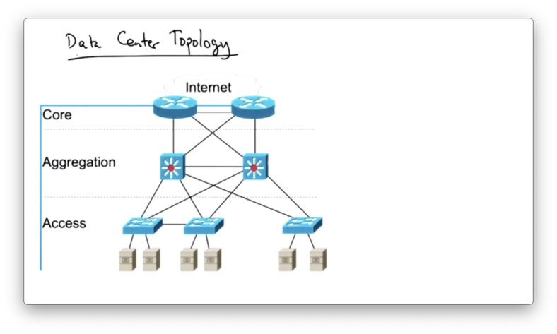
The access layer connects the servers themselves, while the aggregation layer connects the access layer and the core layer provides the connection to the larger internet.
Historically, the core of the network has been connected with layer three, but modern data centers are increasingly being connected entirely over layer two.
Using a layer two topology makes it easier to perform migration of services from one part of the topology to another since these services would not need to be assigned new IP addresses when they are moved.
This approach also makes it easier to load balance traffic.
On the other hand, a monolithic layer two topology makes scaling difficult, since now we have tens of thousands of servers on a single flat topology.
Layer two addresses are not hierarchical, so the forwarding tables in these network switches can't scale as easily because they can't take advantage of the natural hierarchy that exists in the topology.
This hierarchy can potentially create single points of failure and links at the top of the topology in the core layer can become oversubscribed.
Modern data center network operators have observed that core links can carry as much as 200x the traffic carried by links towards the bottom of the hierarchy.
Data Center Topologies
The scale problem arises in data centers because there are tens of thousands of servers on a "flat" layer two topology.
Every server in the network has a topology-independent hardware address and so, by default, every switch in the topology has to store a forwarding table entry for every MAC address.
One solution is to introduce pods. Each server in a pod is assigned a pseudo MAC address in addition to their "real" MAC address.
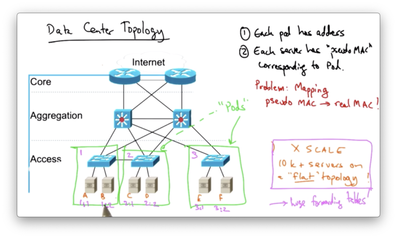
With pods, switches in the data center no longer need to maintain forwarding table entries for every host, but rather only need entries for reaching other pods in the topology.
The receiving switch at the top of each pod will have entries for all of the servers inside that pod, but they don't need to maintain entries for MAC addresses for servers outside of their pod.
In such a data center topology, the hosts are unmodified, so they will still respond to things like ARP queries with their real MAC addresses.
We need a way to intercept queries like this in order to respond with pseudo MAC addresses. In addition, we need a way to map pseudo MAC addresses to real MAC addresses.
When a host issues an ARP query, the query is intercepted by the switch at the top of the pod. Instead of flooding that query to the other pods, the switch forwards it to the fabric manager.
The fabric manager responds with the pseudo MAC address corresponding to the IP address in question.
The querying host then sends the frame with destination pseudo MAC address, and switches in the topology can forward that frame to the appropriate pod corresponding to the pseudo MAC address of the destination server.
Once the frame reaches the destination pod, the switch at the top of the pod can then map the pseudo MAC address back to the real MAC address, and the destination server receives a frame with its "real" MAC address as the destination.
Data Center (Intradomain) Traffic Engineering
Existing data center topologies provide extremely limited server-to-server capacity because of the oversubscription of the links at the top of the hierarchy.
In addition, as services continue to be migrated to different parts of the data center, resources can become fragmented, which can significantly lower utilization.
For example, if a service is broken up across VMs running in different locations of the data center, the service might have to unnecessarily send traffic across the data center topology hierarchy in order to process its workload, thus significantly lowering utilization and cost efficiency.
Reducing this type of fragmentation can result in complicated layer two or layer three routing reconfiguration.
Instead, we'd like to have the abstraction of one big layer two switch, an abstraction provided by VL2
VL2 achieves layer two semantics across the entire data center topology using a name-location separation and a resolution service that resembles the aforementioned fabric manager.
To achieve uniform high capacity between the servers and balance load across links in the topology, VL2 relies on flow-based random traffic indirection using valiant load balancing.
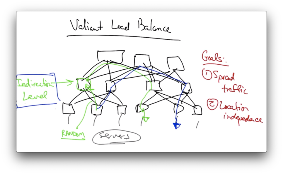
Valiant Load Balancing
The goals of valiant load balancing in the VL2 network are to spread traffic evenly across the servers and to ensure that traffic load is balanced independently of the destinations of the traffic flows.
VL2 achieves this by inserting an indirection level into the switching hierarchy.
When a switch at the access layer wants to send traffic to a destination, it first selects a switch at the indirection level to send the traffic at random.
This intermediate switch then forwards the traffic to the ultimate destination depending on the destination MAC address of the traffic.
Subsequent flows might pick different indirection points for the traffic at random.
The notion of picking a random indirection point to balance traffic more evenly across the topology comes from multiprocessor architecture design, and has recently been rediscovered in the context of data centers.
Jellyfish Data Center Topology
The goals of jellyfish are to achieve high throughput - to support big data, for example - and incremental expandability, so network operators can easily add or replace servers or switches.
For example, large companies like Facebook are adding capacity on a daily basis, and commercial products make it easy to provision servers in response to changing traffic load.
However, it is hard to change the network topology in response to changing traffic load, because the structure of the data center network constrains expansions.
For example, a hypercube configuration requires 2^k switches where k is the number of servers. Even more efficient topologies, such as a fat tree, requires switch counts that are quadratic in the number of servers.
Jellyfish Random Regular Graph
Jellyfish's topology is a random, regular graph.
A regular graph is a graph where each node has the same degree, and a random, regular graph is uniformly sampled from the space of all regular graphs.
In Jellyfish, the graph nodes are switches.
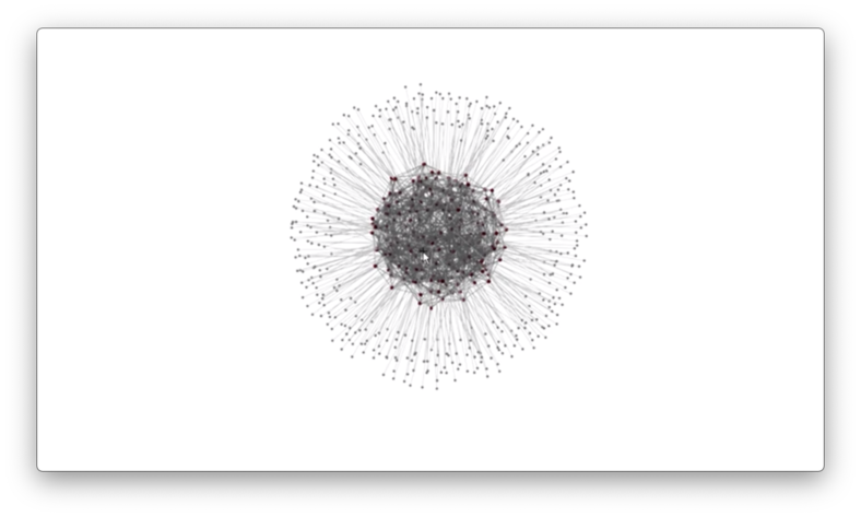
Here is a visualization of a jellyfish random graph parameterized by 432 servers, 180 switches, and a fixed degree of 12.
Jellyfish's approach is to construct a random graph at the Top of Rack (ToR) switch layer.
Every ToR switch i has some total number of ports k_i, of which it uses r_i to connect to other ToR switches. The remaining k_i - r_i ports are used to connect servers.
With n racks, the network supports n * (k_i - r_i) servers.
The network is a random regular graph, denoted as RRG(N, k, r).
Constructing a Jellyfish Topology
To construct a jellyfish topology, take the following steps.
First, pick a random switch pair with free ports for which the switch pair are not already neighbors.
Next, join them with a link and repeat this process until no further links can be added.
If a switch remains with greater than or equal to two free ports - which might happen during the incremental expansion by adding a new switch - the switch can be incorporated into the topology by removing a random existing link and creating a link to that switch.
The jellyfish topology can achieve increased capacity by supporting 25% more servers.
This higher capacity is achieved because the paths through the topology are shorter than they would be in a fat tree topology.
Consider the following topology with 16 server, 20 switches and a degree of 4.
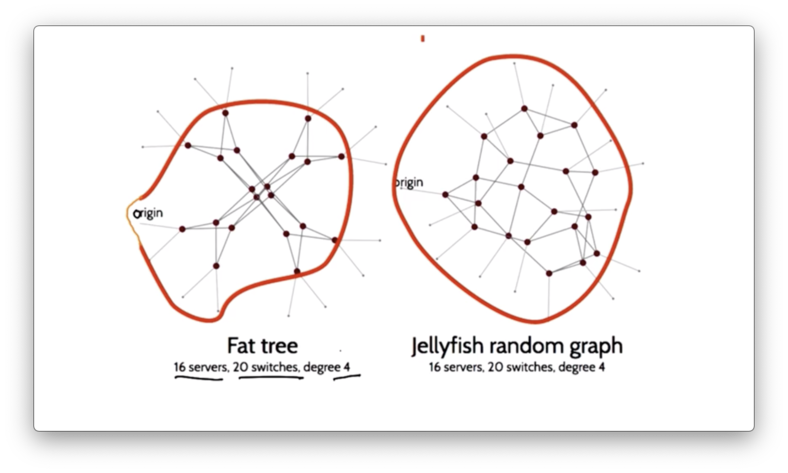
In the fat tree topology, only four out of sixteen servers are reachable by five hops. In the jellyfish random graph, twelve out of sixteen servers are reachable in five hops.
While jellyfish shows some promise, there are still some open questions.
For example, how close are random graphs to optimal in terms of the optimal throughput that could be achieved with a given set of equipment?
Second, how do we connect topologies where switches are heterogenous, with different numbers of ports or different link speeds?
From a system design perspective, the random topology model can create problems with physically cabling the data center network.
There are also questions about how to perform routing and congestion control without the structure of a conventional data center network.
OMSCS Notes is made with in NYC by Matt Schlenker.
Copyright © 2019-2023. All rights reserved.
privacy policy