Assessing a Learning Algorithm

A Closer Look at KNN Solutions

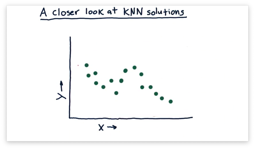
Assume we have the following training examples plotted below, and we want to use the KNN algorithm to provide predictions for new observations.

Now suppose we query the KNN model at the following point, near $x = 0$, using the three nearest neighbors to make our prediction.

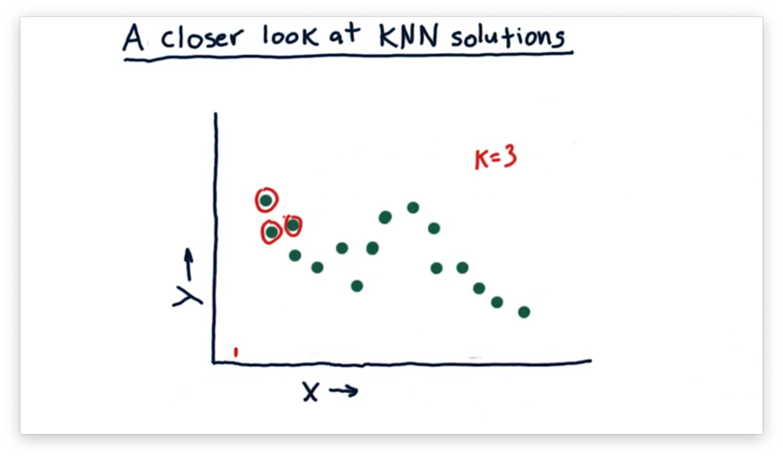
We calculate the predicted $y$ value for this $x$ as the mean of the $y$ values of these three neighbors. As $x$ gets larger, the set of nearest neighbors, and therefore the predicted $y$ value, shifts. We can plot the predicted $y$ values throughout the following continuous range of $x$ values.

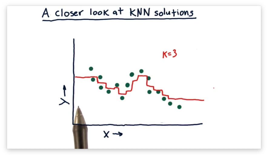
A helpful feature of this model is that it doesn't overfit the data. Since we consider multiple neighbors for each prediction, a prediction is never disproportionately influenced by a single training example.

However, this model is not without its shortcomings. For example, we see flat lines at either end of the plot. After a certain point, the model returns the same prediction for any $x$ because the neighbors don't change. In other words, the model is unable to extrapolate any trends present in the data.

What Happens as K Varies Quiz

Consider the following three models, each generated using a different value for $K$.

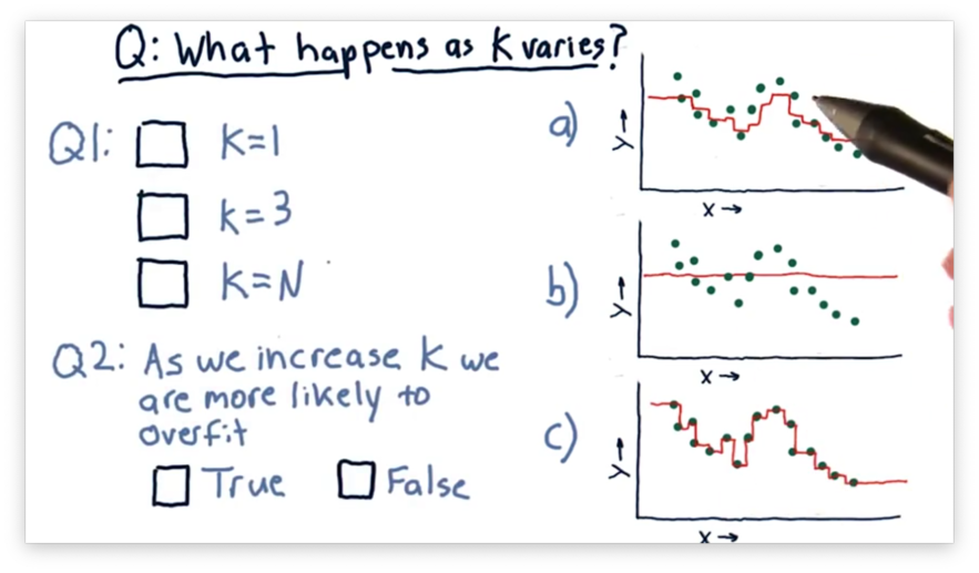
Our first task is to match the value of $K$ with the corresponding plot. Our second task is to decide whether we increase the chances of overfitting as we increase $K$. An overfit model matches the training set very well but fails to generalize to new examples.

What Happens as K Varies Quiz Solution

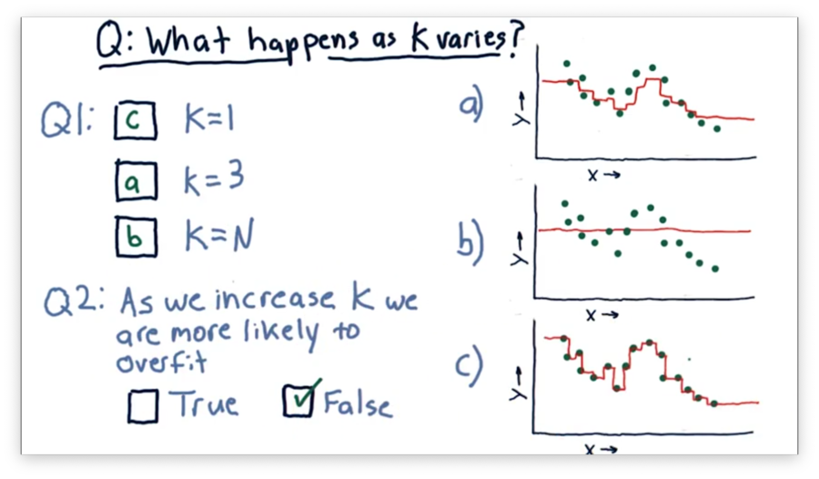
Let's consider the case where $K = 1$. In this case, the model passes through every point $P$ directly, since near $P$, the only point that has any influence is $P$.

Now consider the case where $K = N$. In this case, every point considers all of the neighbors. Thus, the generated model is a straight line passing through the mean of the $y$ values of all the points.

Of course, when $1 < K < N$, the graph lies between these two extremes. For $K = 3$, the graph roughly follows the points without passing through them directly.

As a result, we see that increases in $K$ decrease the probability of overfitting.

What Happens as D Varies Quiz

Consider the following three polynomial models. The difference between each model is the degree of the polynomial $d$.

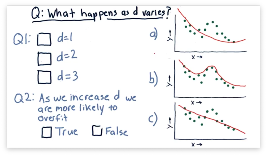
Our first task is to match the value of $d$ with the corresponding plot. Our second task is to decide whether we increase the chances of overfitting as we increase $d$.

What Happens as D Varies Quiz Solution

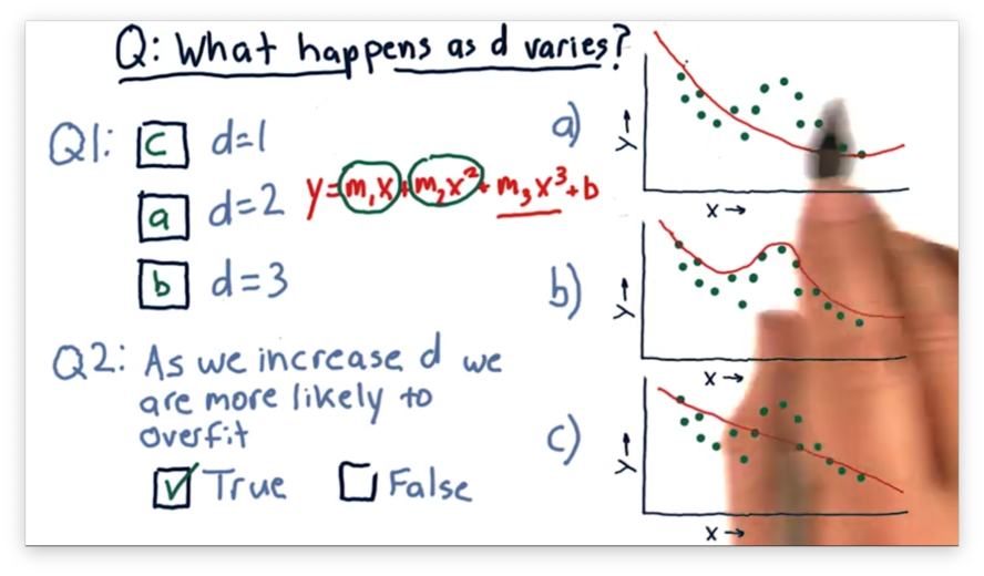
A polynomial of degree one matches the equation $y = m_1x + b$, which is the equation of a line and corresponds to the third plot.

A polynomial of degree two matches the equation $y = m_1x + m_2x^2 + b$, which is the equation of a parabola and corresponds to the first plot.

A third-order polynomial matches the equation $y = m_1x + m_2x^2 + m_3x^3 + b$, which corresponds to the second plot.

We see that as we increase $d$, our model begins to follow the points more closely. Indeed, it can be shown that for $N$ points, a parabola of degree $N$ exists that passes through each point.

Notice that for each of these models, we can extrapolate beyond the data given. This ability to extrapolate is a property of parametric models that instance-based models lack.

Metric 1: RMS Error

We've looked at different graphs of models and visually evaluated how well they fit sets of data. A more quantitative approach to measuring fit is to measure error.

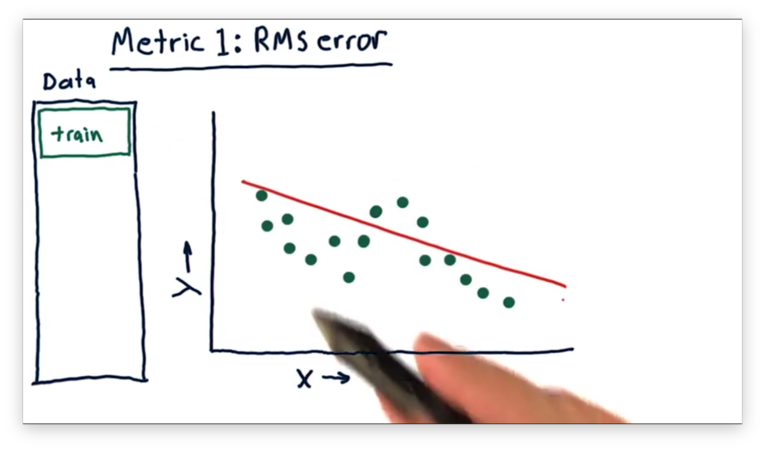
Let's assume we want to build a linear model from the following data.

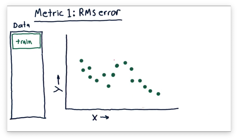
The model might look something like this.

We can assess this model at each real data point $d$ and measure the difference between the $y$-value of $d$ and the $y$-value of the model for the $x$ value of $d$. This difference is the error.

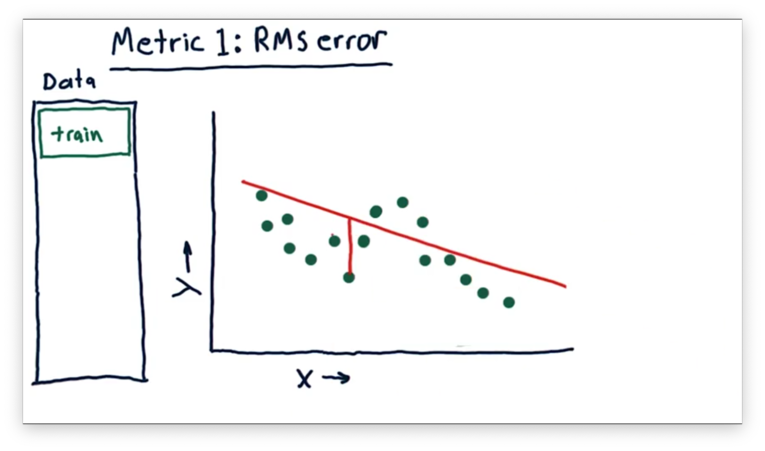
Accordingly, we have an error for every single data point in our data set.

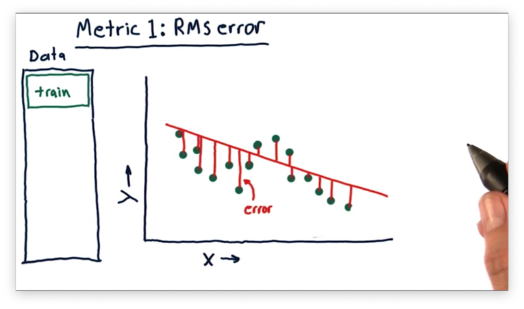
A common type of error is the root-mean-square error (RMSE), which we compute by taking the square root of the mean of the squared errors for each point.

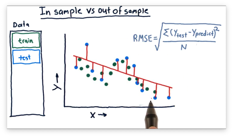
Formally, given a model fit to $N$ data points, each with an error $e_i$, we can calculate RMSE as:

The RMSE formulation gives us an approximation of the average error, although it emphasizes larger errors slightly more than smaller ones.

In Sample Vs. Out of Sample

Remember from our KNN discussion that it's possible to build models that can perfectly fit an arbitrary data set. In other words, we can create a model that has virtually zero error against our training set.

As a result, it doesn't make sense to evaluate our model against the data on which it trained. Instead, we train our model on one set of data and test it on another, previously unseen set of data: the test set.

We minimize the in-sample error between the training set and the model during training. We then compute the out-of-sample error between the test set and the model to evaluate how well the model generalizes to new data.

Which is Worse Quiz

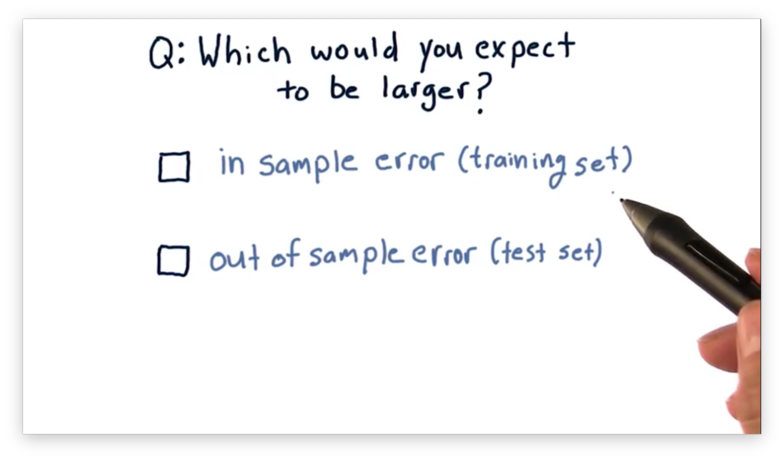
Suppose we just built a model. Which error would you expect to be larger: in-sample or out-of-sample?

Which is Worse Quiz Solution

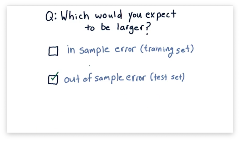
In general, the out-of-sample error is worse than the in-sample error.

Cross Validation

Usually, when researchers are evaluating a model, they split their data into two sets. 60% of the data goes into a training set, and the remaining 40% goes into a test set.

We can think of the process of training and testing a model as a trial. In many cases, a single trial is sufficient to assess a model.

One problem researchers sometimes encounter, however, is that they don't have enough data to analyze their model effectively. They can mitigate this problem by partitioning their data set into different subsets such that they can run multiple trials.

For example, we can slice our data set into five equal partitions. In trial one, we train on the first four slices and test on the fifth. In trial two, we train on the last four slices and test on the first. We can follow this approach to generate a total of five unique train/test splits from our single set of data.

Roll Forward Cross Validation

Cross-validation is a great tool, but typically doesn't fit financial data applications well, at least in the form we've seen so far.

In financial applications, we are typically working with temporal data, and arbitrary selection of training and testing sets can create a situation where our testing data predates our training data.

In other words, we might find ourselves training on data from the relative future and testing on data from the relative past. Any future bias like this can lead to unrealistically optimistic results, so we need to avoid it.

We can avoid this bias with roll forward cross-validation. In roll forward cross-validation, we constrain the selection of training and testing sets such that training data always comes before test data. Even with these constraints, we can still subset our data to create multiple train/test trials.

For example, let's suppose we slice our data set into five equal partitions. In trial one, we train on the slice one and test one slice two. In trial two, we train on slice two and test on slice three. We can follow this approach to generate a total of four unique train/test splits from our single set of data.

Metric 2: Correlation

Another way to evaluate the accuracy of a regression algorithm is to look at the relationship between predicted and observed values of our dependent variable, $y$.

Let's suppose we have a model $M$ and a set of testing data containing $X_{test}$ and $Y_{test}$. We can query $M$ with $X_{test}$, and it will return a set of predictions $Y_{predict}$. We can then compare the predicted values against the ground truth.

We compute the correlation between $Y_{test}$ and $Y_{predict}$ to quantitatively measure the relationship between the two sets of variables. Correlation values range from -1 to 1, where -1 indicates a perfect inverse relationship, 1 indicates a perfect positive relationship, and 0 indicates no relationship.

Ideally, we would want to see a correlation between $Y_{test}$ and $Y_{predict}$ of precisely 1, which would indicate that the two sets of data are identical; that is, our model made no prediction errors.

Given two ndarrays n1 and n2 of identical shapes, we can compute the correlation between them like:

np.corrcoef(n1, n2)

Documentation

• numpy.corrcoef

Correlation and RMS Error Quiz

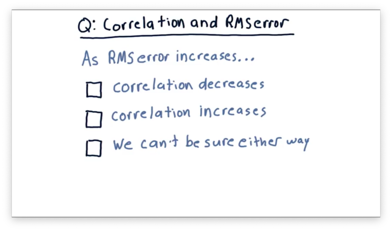
Let's think about the relationship between RMS error and the correlation between $Y_{test}$ and $Y_{predict}$. Which of the following statements is true?

Correlation and RMS Error Quiz Solution

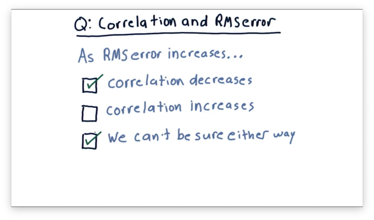
In most cases, correlation decreases as RMS error increases. However, it is possible to construct examples where correlation increases as RMS error increases.

Overfitting

Let's consider a parameterized polynomial model $M$. We want to increase the degree of $M$ steadily - adding an $x$ term, an $x^2$ term, an $x^3$ term, and so on - and understand how the error changes in response.

We can look at the in-sample error first. When $d$ is smallest, our error is highest, and as we increase $d$, our error drops. As $d$ approaches the number of items $N$ in our data set, our error can approach zero.

Let's look at the out-of-sample error next. Remember that we always expect out-of-sample error to be greater than or equal to in-sample error.

When $d$ is small, our out-of-sample error is likely to be very close to our in-sample error. However, as $d$ increases, the out-of-sample error gets larger. In other words, a model with more factors can fit the training data better at the expense of fitting the test data. Indeed, at large values of $d$, we might see sharp increases in out-of-sample error.

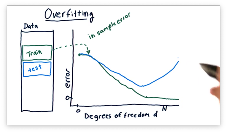
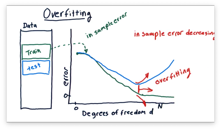
We can define overfitting as the range in which adding additional factors to our model results in a decrease in in-sample error but an increase in out-of-sample error.

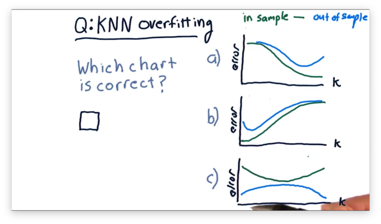
Overfitting Quiz

Let's consider overfitting in KNN and how in-sample and out-of-sample error changes as $K$ increases from 1 to the number of items $N$ in a data set.

Which of the following plots correctly represents the shape of the error curves that we would expect for both types of error as we increase $K$?

Overfitting Quiz Solution

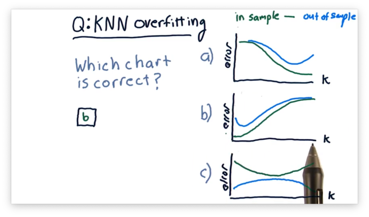
Remember that KNN models are least generalized when $K = 1$. In other words, when $K = 1$, the model predicts each training point in the data set perfectly but fails to predict testing points accurately. As a result, KNN models overfit when $K$ is small.

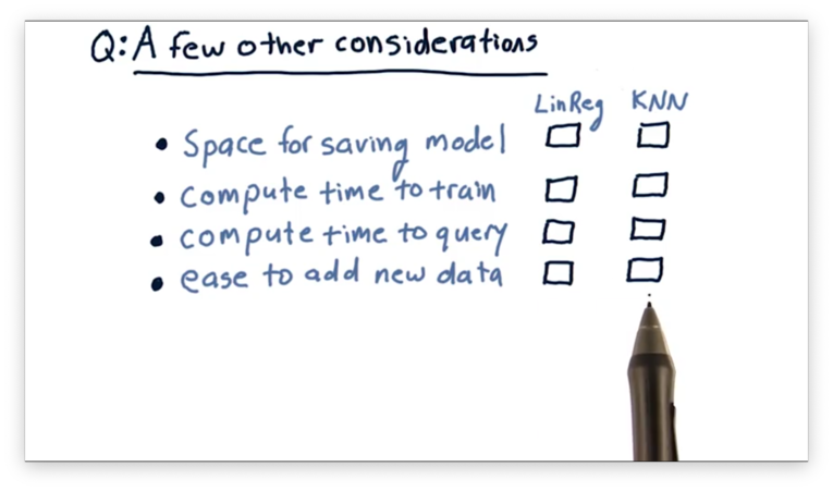
A Few Other Considerations Quiz

There are a few other factors worth considering when evaluating a learning algorithm. For each of the following factors, which of the two models has better performance?

A Few Other Considerations Quiz Solution

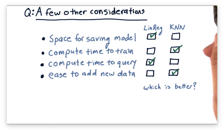
Linear regression models require less space for persistence than KNN models. A linear regression model of degree four can be described in as few as four integers, while a KNN model must retain every single data point ever seen.

KNN models require less compute time to train than linear regression models. In fact, KNN models require zero time to train.

Linear regression models process queries more quickly than KNN models. The query time for a linear regression model is constant. The query time for KNN models grows with the number of queries, as previously queried data points are added to the data set and must be examined in subsequent queries.

Adding new data is quicker in KNN than in linear regression. Incorporating new data into a model requires retraining the model, but, as we just saw, the training time for a KNN model is zero.