Optimizers: Building a Parameterized Model

What is an Optimizer

An optimizer is an algorithm that searches the input space of a target function for values that drive the output of that function towards some goal.

We use optimizers for several different purposes.

For one, we use optimizers to find minimum values for functions. For example, given a function $f(x) = x^2 + x^3 + 5$ , we can use an optimizer to find an $x$ such that $f(x)$ is as small as possible.

Additionally, we use optimizers to find the parameters of models we want to build from data. For example, we might collect data that captures a relationship between two variables, and we can use optimizers to find the coefficients of a polynomial that describes that relationship.

Finally, and from a more practical perspective, we can use optimizers to refine stock allocations in portfolios. In other words, an optimizer can help us decide what percentage of our funds we should allocate to each stock.

Using an optimizer involves three main steps. First, we define the function that we want to optimize. For example, if we want to optimize $f(x) = x^2 + x^3 + 5$ , we can define the following function in Python:

def func(x):
    pow(x, 2) + pow(x, 3) + 5

Second, we declare the initial arguments to the function. Ideally, we want to use arguments that are close to the optimal arguments, but if we have no idea what those values should be, random arguments are sufficient.

Finally, we call the optimizer, passing in the function and the initial arguments. The optimizer calls the function many times, slightly changing the arguments each time until it finds a solution.

Minimization Example

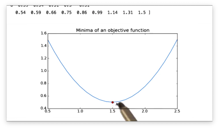
Let's take a look at the function $f(x) = (x - 1.5)^2 + 0.5$ , which is graphed below.

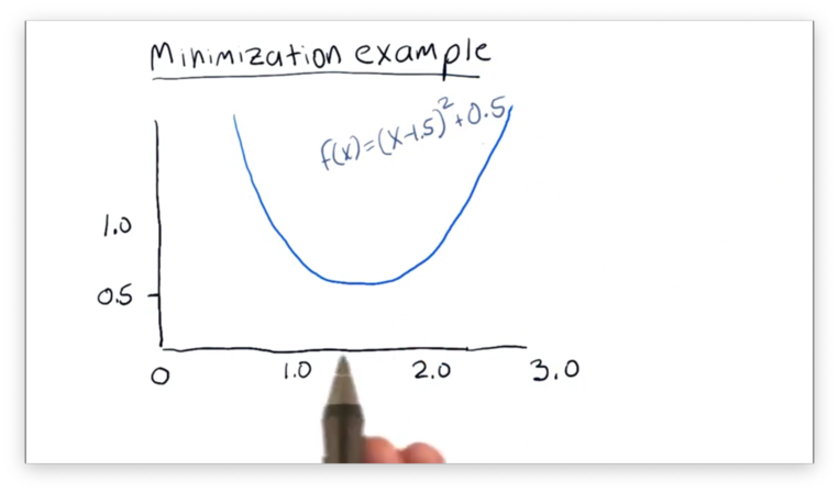
From the graph, we can see that the function is centered horizontally about the line $x = 1.5$ with a global minimum at $(1.5, 0.5)$ . While we can find this minimum fairly intuitively, a minimizer, of course, cannot.

We must supply the minimizer with an initial value of $x$ and let it iteratively move closer to the minimum. Let's suppose we tell the minimizer to start with a value of $x=2$ .

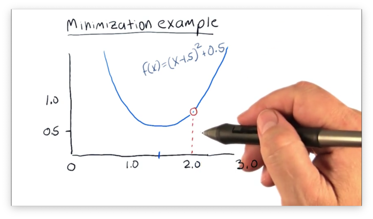
The first thing the minimizer does is evaluate $f(2)$ , which equals 0.75. It then tests two very nearby values - one greater than 2 and one smaller than 2 - and computes the slope of the line connecting those two points.

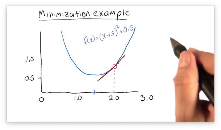
The slope of the line connecting the two points gives the minimizer insight into how to adjust $x$ . Since the slope is positive, increases in $x$ result in increases in $f(x)$ . Since the minimizer wants to minimize $f(x)$ , it knows to decrease $x$ .

This iterative process - adjusting $x$ , computing $f(x)$ , finding the slope, and then increasing or decreasing $x$ appropriately - is known as gradient descent. Read more about gradient descent here.

After several rounds of gradient descent, the minimizer finds the minima at $(1.5, 0.5)$ and ceases its search.

Minimizer in Python

Let's optimize the function $f(x) = (x - 1.5)^2 + 0.5$ using Python. For this task, we will need to import a new module, scipy.optimize:

import scipy.optimize as spo

We can define $f(x)$ in Python with the following code. Note that we add a print line so we can trace the iterations of the minimizer.

def f(x):
    y = (x - 1.5)**2 + 0.5
    print("X = {}, Y = {}".format(X, Y)) # for tracing
    return y

Now we turn to the minimize function of the scipy.optimize module. Generally, we can minimize a function f starting with an initial value x like so:

spo.minimize(f, x)

In our case, we call minimize with an initial value of 2.0. Additionally, we pass a value for the method parameter, which specifies the type of algorithm used to minimize f.

minimized = spo.minimize(f, 2.0, method="SLSQP", options={'disp': True})

Note that we also supply the disp option set to True which adds some additional print messages.

Perhaps surprisingly, the value of minimized is not a number, but an object. We can access the value of x and the corresponding, minimized value of f(x) like so:

minimized.x # x
minimized.fun # f(x)

If we run our optimizer and print out our minimized values, we see the following output.

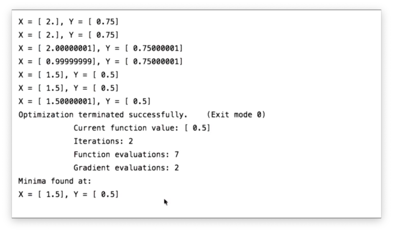
We see the iterative progress of the minimizer thanks to the print statements we placed in f. We see some additional output - a result of the {'disp': True} option - that provides information on the number of iterations and function evaluations required during the minimization process. Finally, we see the minimum.

To visually verify that the minimizer found the correct value, we can plot f and place a point at the value of (minimized.x, minimized.fun).

Documentation

scipy.optimize.minimize

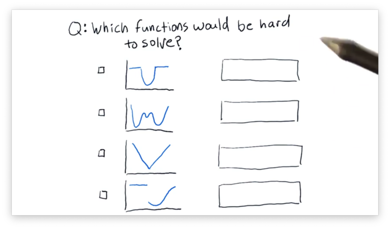
How to Defeat a Minimizer Quiz

Which of the following functions would be hard for the minimizer to solve?

How to Defeat a Minimizer Quiz Solution

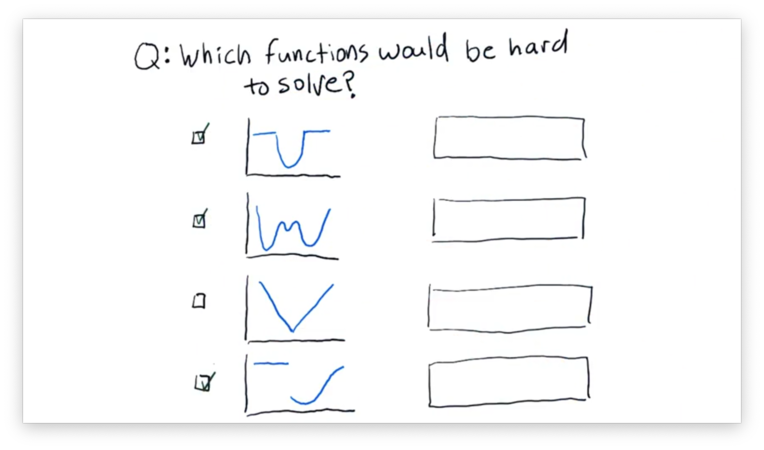
The first graph is hard because of the "flat" areas on either side of the parabola. A minimizer testing a point in the middle of this area wouldn't be able to find any gradient to follow, so it wouldn't know how to adjust the value it was currently testing.

The second graph is hard because it has several local minima that aren't necessarily the global minimum. A minimizer might "get stuck" in a local minimum, even though a more significant, global minimum exists.

The fourth graph is challenging both because of the "flat" area and the discontinuity between the two halves.

Convex Problems

Minimizers are best at minimizing convex functions. According to Wikipedia:

In mathematics, a real-valued function defined on an n-dimensional interval is called convex if the line segment between any two points on the graph of the function lies above or on the graph.

In other words, pick two points on the graph of a function and draw a line connecting the points. If the graph of the function does not intersect that line, then the function is convex between those points.

Let's look at three examples.

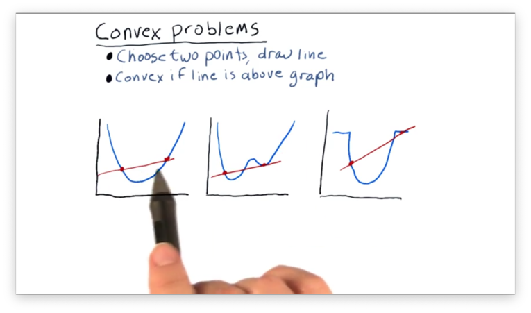
We can see that the first function is convex between the two points we have selected (actually, it's convex everywhere).

We can see that the second and third functions are not convex between the two points as a portion of the graph in each lies above the line between the points.

As a result, we can observe some properties required for convexity. If a function is to be convex, it must have only one local minimum - the global minimum - and cannot have any "flat" regions with zero slope.

If the function you want to minimize is convex, the algorithms we examine will find the minimum quickly and easily. Algorithms that can find minima for non-convex functions exist, but they require a bit of randomness and aren't guaranteed to find the global minimum.

So far, we have looked at functions that only have one dimension in $x$ , such as the parabola we minimized previously. Consider the following graph, which depicts a function that has two dimensions in $x$ .

The good news is that minimizers can solve these multi-dimensional problems with gradient descent just as effectively as they can solve one-dimensional problems.

Building a Parameterized Model

Let's look at a function that we have all seen before:

f(x) = mx + b

This function, which is also the equation for a line, has one argument, $x$ , and two parameters: $m$ and $b$ .

Note: For convenience, in our code we refer to $m$ and $b$ and $C_0$ and $C_1$ , respectively.

Now let's look at some data points. Let's say we are budding meteorologists and want to understand the relationship between humidity and rainfall. We collect daily humidity measurements and observe how much it rains, and we create the following plot.

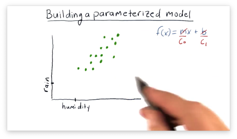
We can see a relationship between humidity and rainfall, and our intuition is that we might be able to model this relationship with a line. The line might look something like this.

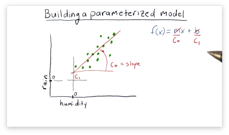
Our task is to find the parameters $C_0$ and $C_1$ that describe the line that best fits our data. Since we are working with minimizers, we need to reframe this problem as a minimization problem.

What is it we are trying to minimize? Let's look at a simpler example.

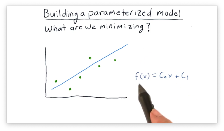
Looking at the graph above, suppose we've collected the data points plotted in green, and we are trying to evaluate how the blue line fits these points.

We can evaluate the line by examining the vertical distance between each point and the candidate line.

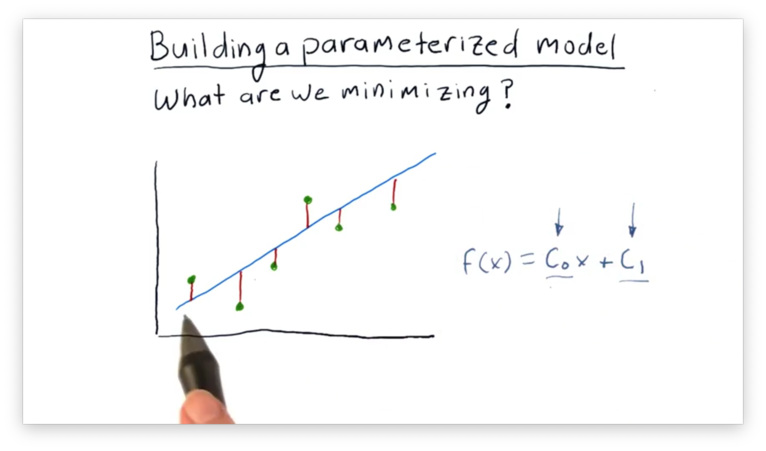
It is these vertical distances, or errors, that we want to minimize.

What is a Good Error Metric Quiz

Let's assume that a point $p_i$ has an error $e_i$ , which is the vertical distance between $p_i$ and the best-fit line currently under consideration. Given a number of such errors $e_0, e_1, ..., e_n$ , which of the following expressions describes the metric we want to minimize?

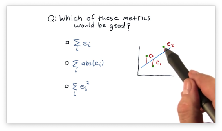
What is a Good Error Metric Quiz Solution

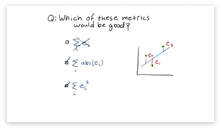
We want to minimize the sum of the errors, but we want to ensure that errors above and below the line do not cancel out. To accomplish this, we need to make each error positive by either squaring it or taking its absolute value.

Minimizer Finds Coefficients

Let's look at the following data.

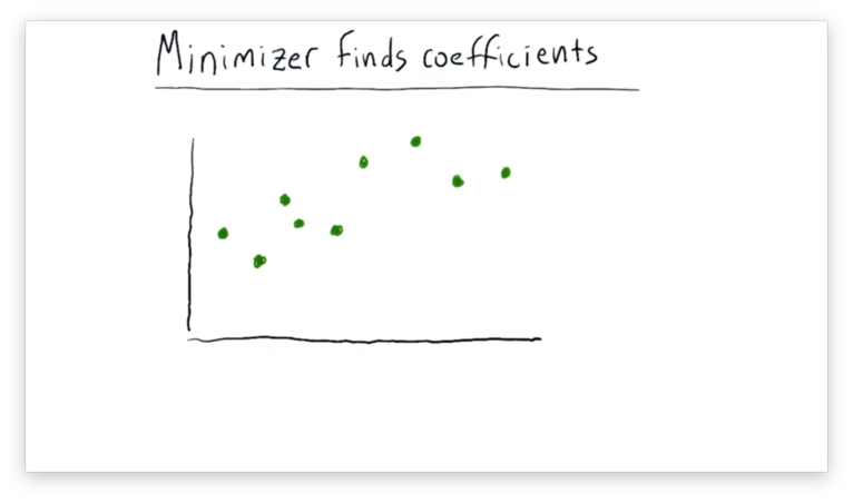
We want to use a minimizer to find the line that best fits this data, so we first have to define a function to minimize. We are going to use the sum of squared error function we saw above, namely:

E = \sum_i{e_i^2}

Additionally, we have to give the minimizer our initial guess for $C_0$ and $C_1$ , and we might choose the values one and zero, respectively. We would give $E$ , $C_0$ , and $C_1$ to the minimizer and let it run from there. The minimizer iteratively adjusts $C_0$ and $C_1$ , observing how $E$ changes with each adjustment, until eventually settling on values of $C_0$ and $C_1$ that minimize $E$ .

Fit a Line to Given Data Points

Let's walk through some example code that generates a best-fit line for a set of data points.

Remember that we are using an optimizer to accomplish this task, so the first thing that we have to do is define the function we want the optimizer to minimize.

This function, which we call error, takes in two arguments: line and data. The line argument is a tuple containing the parameters - $C_0$ and $C_1$ - of the current line under consideration. The data argument is a two-dimensional array containing x- and y-values from our data set.

We can implement error in Python like so:

def error(line, data):
 return np.sum((data[:, 1] - (line[0] * data[:, 0] + line[1])) ** 2)

Let's walk through what this function does. First, for every x-value given, we compute the corresponding y-value using the equation of the best-fit line:

line[0] * data[:, 0] + line[1]

Next, we subtract these expected values from the observed y-values in our data:

data[:, 1] - (line[0] * data[:, 0] + line[1])

Third, we square the differences:

(data[:, 1] - (line[0] * data[:, 0] + line[1]) ** 2)

Finally, we sum the squared differences:

np.sum((data[:, 1] - (line[0] * data[:, 0] + line[1])) ** 2)

Now that we have error, the function we want to minimize, let's test our minimizer. Our test consists of three steps, shown in Python below.

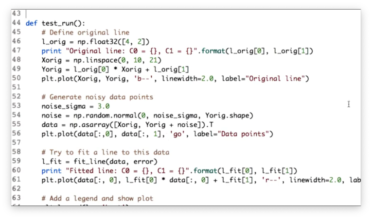
First, we define the line that we want the minimizer to discover. The variable l_org holds the parameters of this line, which has a slope of 4 and a y-intercept of 2. We create an array of evenly-spaced x-values Xorig using np.linspace and an array of the corresponding y-values Yorig. We plot Xorig against Yorig to draw our line.

Second, in an attempt to "fool" the minimizer, we add some random noise to the y-values in Yorig. We can generate this noise by sampling a Gaussian distribution with a mean of zero and a standard deviation of three. We combine Xorig with the new, noisy y-values into an array data, which we plot.

Third, we call the fit_line function, passing in data and error, which runs the minimization task and gives us the coefficients of the best fit line. Finally, we plot this line.

Let's look at fit_line.

def fit_line(data, error):
 l = np.float32([0, np.mean(data[:, 1])])

 # Plotting code for initial guess omitted

 result = spo.minimize(error, l, args=(data,), method="SLSQP", options={'disp': True})

 return result.x

First, we define our initial guess l for the parameters that minimize error. We choose a slope of 0 and a y-intercept equal to the mean of the y-values in data.

Next, we pass error and l to spo.minimize.

Remember that error takes two arguments: the parameters of the line and the data from which it computes the error. By default, the minimizer passes the line parameters to error. However, we have to manually tell the optimizer to pass data as well, which is why we specify the args parameter in the call to spo.minimize.

Additionally, we specify the method and pass in some verbosity options.

We can finally run our test, and we see the following chart.

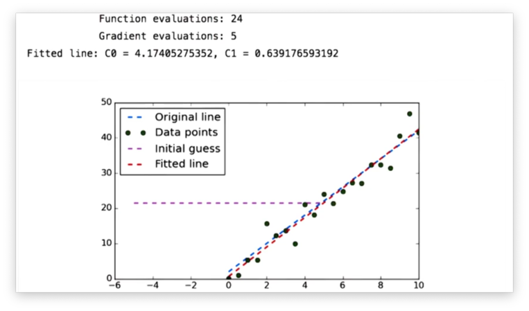
Our original line is the blue line, and the green dots are the noisy data we generated from points on that line. The purple line is the original guess that we passed to the minimizer. The minimizer fit the red line to the data, and, indeed, it is quite close to the blue line.

Documentation

And it Works for Polynomials Too

We can fit even more complicated functions to data, such as the polynomial we fit to the data below.

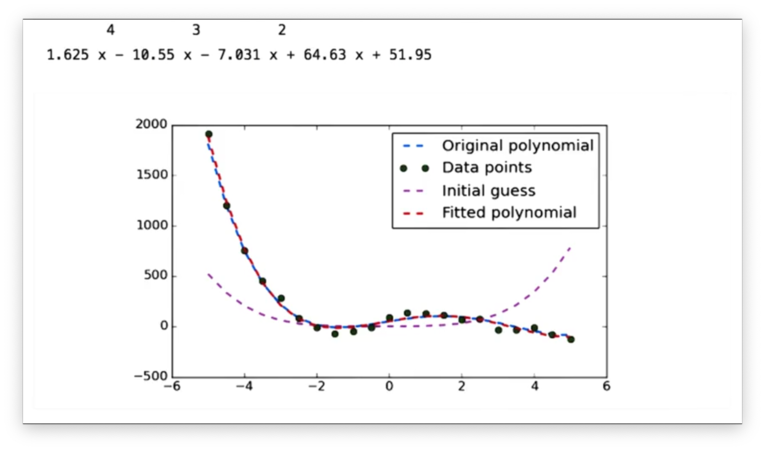
Let's look at the output from the minimizer that generated this polynomial.

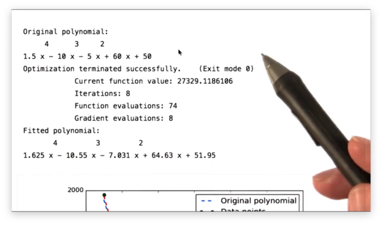
We can see that the coefficients of the fitted polynomial are very similar to those of the original polynomial.

Let's look at how we structured this minimization problem in Python. First, our error function changed slightly:

def error(C, data):
  return np.sum((data[:, 1] - np.polyval(C, data[:, 0])) ** 2)

Since we are fitting a polynomial to our data, we can no longer use the equation of a line to generate expected y-values from our x-values. Instead, we use np.polyval.

Additionally, our fit function, now called fit_poly, is different:

def fit_poly(data, error, degree=3)
  Cguess = np.poly1d(np.ones(degree + 1))

  # Plotting code for initial guess omitted

  result = spo.minimize(error, Cguess, args=(data,), method="SLSQP", options={'disp': True})

  return np.poly1d(result.x)

Notably, our initial guess is no longer an array containing two parameters, but rather an array of all ones, of length degree + 1. Additionally, we turn this array into an object representing the polynomial it parameterizes using np.poly1d.

Machine Learning Trading