Machine Learning Trading
Technical Analysis
13 minute read
Notice a tyop typo? Please submit an issue or open a PR.
Technical Analysis
Technical Vs. Fundamental Analysis
There are two broad categories of approaches to use when choosing stocks to buy or sell: fundamental analysis and technical analysis.
Fundamental analysis involves looking at aspects of a company in order to estimate its value. Fundamental investors typically look for situations where the price of a company is below its value.
Technical analysis, on the other hand, isn't concerned with the underlying value of a company; instead, technicians look for patterns or trends in a stock's price.
Characteristics
One of the most important things to remember about technical analysis is that it considers only price and volume data, as opposed to fundamental analysis, which looks at factors such as earnings, dividends, cash flows, book value, and more.
In technical analysis, we look back at historical price and volume data to compute statistics, also known as indicators. These indicators serve as heuristics that might hint at buying or selling opportunities.
There is significant criticism of the technical approach, and many people consider it an inappropriate method for investing because it doesn't consider the value of the company. Instead, we might think of technical analysis as a trading approach, rather than an investing approach.
However, there are reasons to believe that technical analysis might have value. There is information in price and price change, as these data points reflect sentiments of buyers and sellers. Especially when the price for a particular stock is moving against the overall market, pricing data and volume can present trading opportunities.
Additionally, while we know that heuristics cannot guarantee outcomes, we also know, from other domains of artificial intelligence, that heuristics are valuable and are frequently used to inform critical decisions.
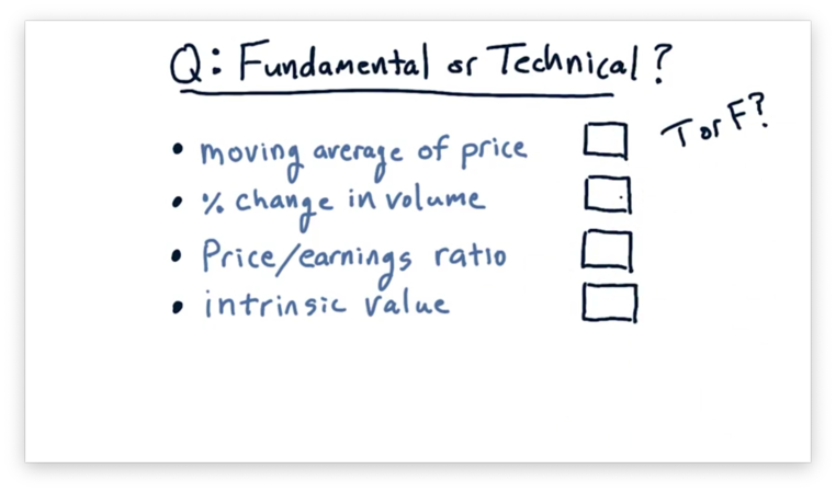
Potential Indicators Quiz
Now that we know some differences between the types of data used for fundamental and technical analysis, let's look at the following four factors. Which of these are fundamental, and which are technical?
Potential Indicators Quiz Solution
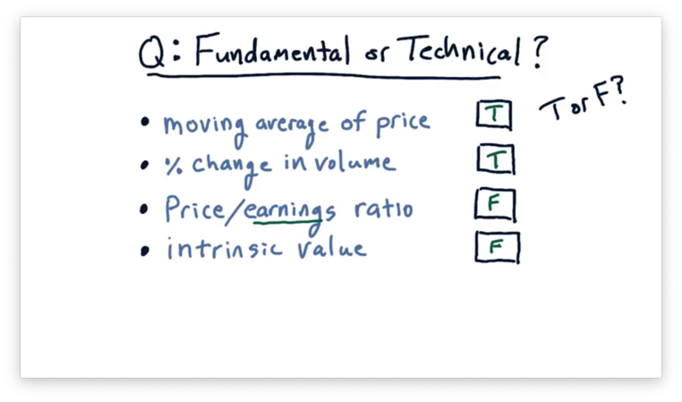
Remember that technical analysis considers only price and volume data, whereas fundamental analysis incorporates other types of data.
The moving average of price and the percent change in volume consider only price and volume, respectively, so they are both technical indicators.
P/E ratio considers both price and earnings, making it a fundamental factor, as well as intrinsic value, which is based on dividends.
When Is Technical Analysis Valuable
Let's consider how we can use technical analysis to derive meaningful information about a stock.
Back in the 1980s and 1990s, when many of the well-known indicators were developed, they may have had reliable predictive power. Since that time, however, more people have been trading according to these indicators. Generally, the more people that follow a particular investing approach, the less value any one investor realizes. As a result, individual indicators are only weakly predictive today.
That being said, combining multiple indicators still adds value. Combinations of three to five technical indicators, in a machine learning context, may provide a much stronger predictive system than just a single indicator.
Technical analysis can also be useful at highlighting contrast; in other words, revealing when two stocks - or one stock and the market - have widely different values for a particular indicator. Such a contrast might be indicative of an actionable opportunity.
Finally, technical analysis generally works better over the short term than over the long term.
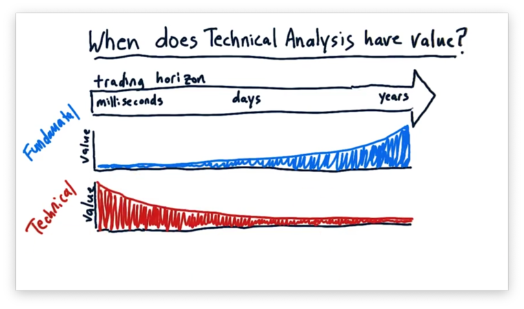
When Is Technical Analysis Valuable, Part Two
To understand the value of technical analysis as compared to fundamental analysis, we need to consider the trading horizon: the amount of time that elapses between buying and selling a stock. Trading horizons can vary from milliseconds to years.
Let's first consider fundamental factors. If we are a high-frequency trading (HFT) fund operating over trading horizons of milliseconds, how much do fundamental factors like P/E ratio and book value contribute to the change in price over these short periods of time?
When we are rapidly executing trade orders, the only factors that matter are those present on the stock exchange, such as price movement and trading volume. For these very short trading horizons, fundamental factors have quite low value.
Let's now consider a trading horizon of years. We know from, for instance, Warren Buffet's success that fundamental factors over long periods of time may have significant value.
For a trading horizon of days, fundamental factors may have some value; in general, the longer the trading horizon, the more valuable fundamental factors are.
Let's now consider technical factors. How valuable is a technical indicator, such as a 20-day momentum, in determining the price of a stock years later? Such indicators have little value when considering a trading horizon of years.
For a very short trading horizon, however, technical analysis can shine. In the span of a few milliseconds, the only factors about a stock that have changed are technical factors, and, as a result, technical analysis can potentially have high value over trading horizons of this size.
For a trading horizon of days, technical factors may have some value; in general, the longer the trading horizon, the less valuable technical factors are.
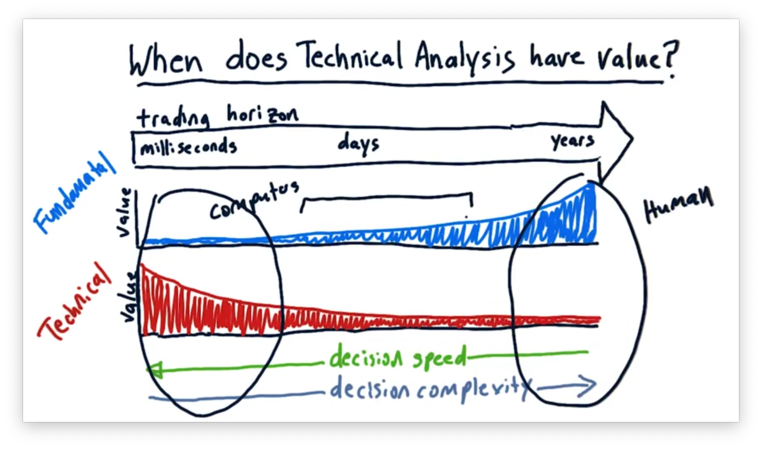
Let's consider the value of decision complexity and decision speed across the range of trading horizons.
Over a period of years, a lot can happen to a company, and, correspondingly, its stock price. As a result, we can appreciate a complex decision-making process for investments with a trading horizon of this length.
Decision speed is not as important when considering investments that we plan to hold for years. Relative to this investment horizon, it doesn't so much matter if it takes us a minute or a day to make an investment decision.
When considering a much shorter trading horizon, decision speed is of utmost importance. If we want to buy and sell stock over the period of milliseconds, we can't take seconds to make decisions. Correspondingly, we also value decision complexity less at a trading horizon of this size.
We can look at this range of trading horizons and think about which regions are more suited for human investors and which are more suited for computational investment.
When trading at very high frequencies, we need to leverage technical analysis to make many simple decisions very quickly. Thankfully, these decisions are often simple enough to capture in computer code. As a result, we often see computers trading over these shorter trading horizons.
Over a longer trading horizon, where decision speed is less of a factor, and the decisions are complex, humans typically outperform computers.
Let's think about the different types of hedge funds we might find in the wild. On the one hand, we might see an HFT-based fund using technical analysis to trade over a millisecond horizon. On the other hand, we might find an insight-driven, human-based hedge fund holding positions for much longer. In between, we often see humans and computers working together.
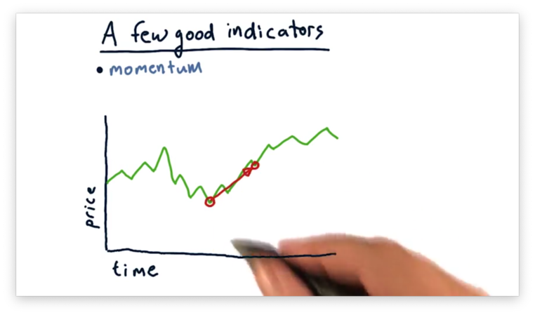
A Few Indicators: Momentum
The first technical indicator that we are going to consider is momentum. Momentum refers to the relative change in price for a stock over a certain number of days.
If we consider the two points on the price chart below, we can see positive momentum.
If we consider these two points, we can see negative momentum.
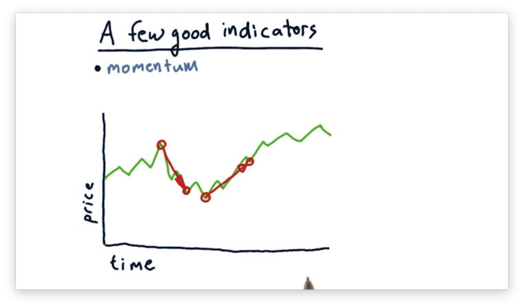
The slope of the line connecting the two points indicates the strength of the momentum, either positive or negative.
We can incorporate momentum into a trading strategy. Many folks choose to buy on positive momentum and sell on negative momentum because they anticipate that the current trend is going to continue.
While we have seen what momentum looks like visually, we need a quantitative representation of momentum that we can use in a machine learning context.
We said that momentum refers to the relative price change over a certain number of days. To calculate momentum, we have to define how many days we want to use. For example, we might consider a five-day momentum that compares prices from five days ago to prices today or a ten-day momentum that uses an equivalent comparison.
Generally, if we want to calculate the -day momentum, , at day , using a sequence of prices, , we can use the following formula.
This formula gives us a number indicating how much the price of a stock has risen or fallen between day and day . We typically see numbers for momentum between -0.5, for a significant price drop, and 0.5, for a significant price jump.
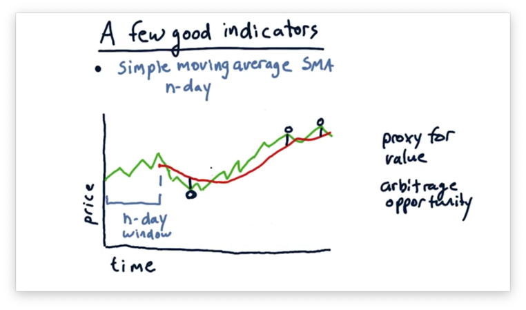
A Few Indicators: Simple Moving Average
Our next indicator is simple moving average (SMA), which, given , computes the average price over the previous days, known as an -day window.
We don't have to compute the SMA for only a single day. Instead, we can repeatedly slide our window forward one day to compute the -day SMA for every day from to today. The plot of such an SMA is shown below.
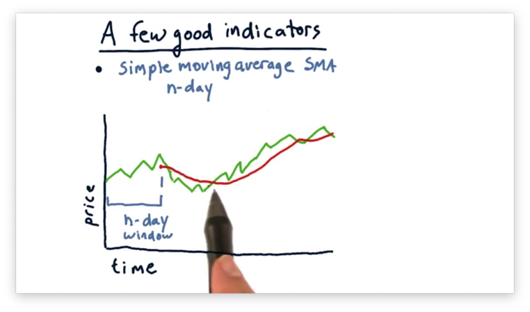
Note that the SMA plot essentially looks like a smoothed version of the price chart. Also, notice that the movement of the SMA data lags that of the pricing data; in other words, the peaks and troughs that appear in the pricing data don't appear in the SMA data for several days.
There are at least two different ways that technicians use simple moving averages in their trading strategies. First, they look for places where the current price crosses through the SMA, as seen below.
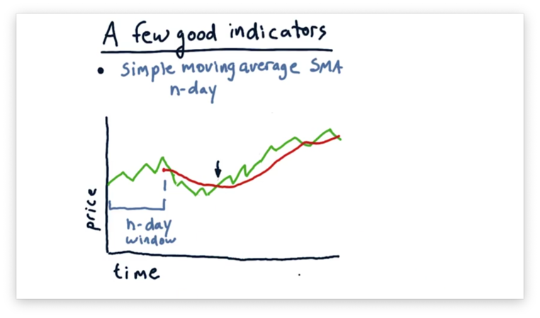
Such crossovers tend to be significant events, especially when is quite large. Coupled with supporting momentum, a crossover might constitute a strong buy or sell signal.
Technicians might also use simple moving average as a proxy for underlying value. In other words, if we calculate the average price over a large enough window, we might be able to estimate the true value of the company.
If we see a large excursion from such a simple moving average, we should expect that the price is going to regress toward that average. Given that knowledge, excursions may present trading opportunities.
For example, we can uncover one potential buy signal and two potential sell signals below by looking at such excursions.
Just as we saw with momentum, a visual representation of simple moving averages is not enough. We need a quantitative representation of SMAs if we are to use them in our machine learning algorithms.
Generally, if we want to calculate the -day simple moving average, , at day , using a sequence of prices, , we can use the following formula.
We can also quantify buy and sell signals.
Similar to momentum, values for SMA typically range from -0.5 to 0.5.
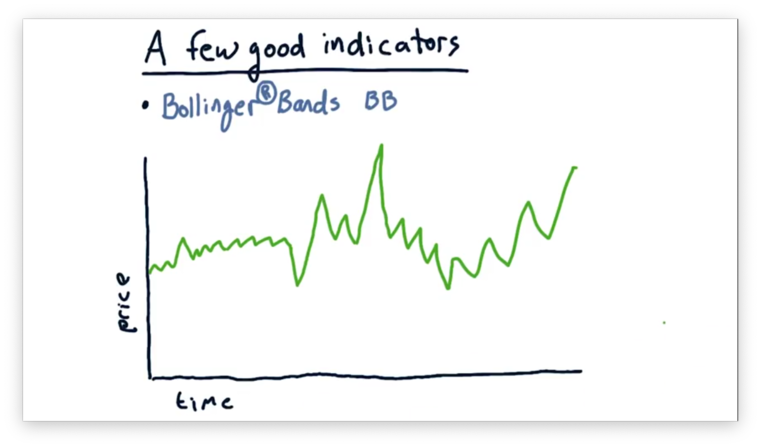
A Few Indicators: Bollinger Bands
Suppose we have the following plot demonstrating the price of a stock over time.
We want to leverage simple moving averages to inform us of potential buying and selling opportunities. Let's add the simple moving average to the plot.
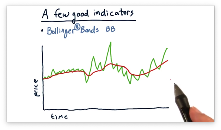
We are trying to decide how much of an excursion from the simple moving average we should use as a trading signal. We might choose a fixed percentage of, say, 1%.
However, as we step forward in time, we see that most of the price movement is at least 1%. According to our static rule, we'd be constantly trading. Clearly, a fixed number is not the way to go.
Our pricing chart shows two distinct regions: one of low volatility and one of high volatility.
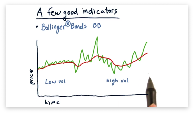
John Bollinger observed that, for a stock experiencing low volatility, we should use a relatively smaller value for our signal, and, for a stock experiencing high volatility, we should use a relatively larger value.
We can accomplish such dynamic signaling using a statistic, derived from the pricing data itself, that captures volatility. Specifically, that statistic is standard deviation. For each day, we can take the standard deviation of the prices that constitute the simple moving average for that day. Given this standard deviation, we typically create Bollinger Bands two standard deviations above and below the simple moving average.
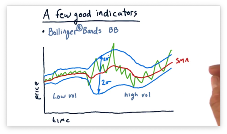
These bands provide a dynamic measure for how much of a deviation we want to see before we respond. The bands are tighter for periods of low volatility, and a relatively smaller excursion is enough to break out of the bands. In periods of higher volatility, the bands are much wider, and we only see crossovers for more aggressive deviations.
We can use Bollinger Bands in our trading strategies. A general rule of thumb is: look for times when the price crosses from the outside of a band to the inside.
For example, observe the following sell signal.
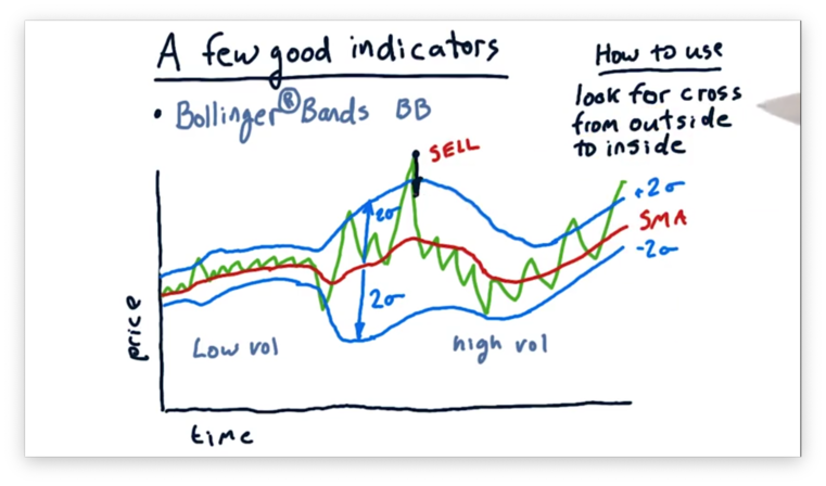
Here we see a large positive excursion from the simple moving average, followed by a Bollinger Band crossover in the direction of the moving average.
From our discussion on moving averages, we said that we expect prices to regress to the moving average, and the crossover event we see above demonstrates such a regression. Since a regression downward to the mean involves a further drop in price, we might consider selling.
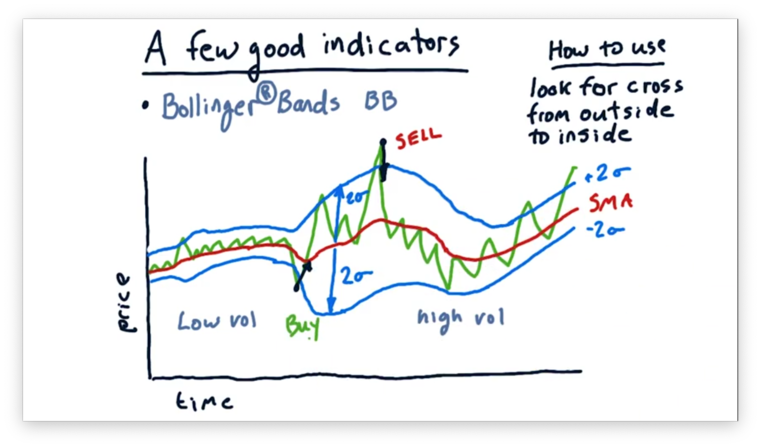
Conversely, when we see price crossing over from the outside to the inside of the bottom band, we might consider buying.
Generally, if we want to calculate the Bollinger Bands, , on a given day, , from a sequence of prices, , using an -day moving average, , we can use the following formula. Note that refers to the standard deviation.
Additionally, we can look at the ratio, , of the current price, less , to the current Bollinger Band, .
We typically see values for between -1.0 and 1.0. In other words, the price rarely breaks out of the Bollinger Bands. Of course, this makes sense, as they are placed two standard deviations outside of the mean.
By comparing the value of over two consecutive days, and , we can quantify buy and sell signals.
Buy or Sell Quiz
Let's consider how we might trade using Bollinger Bands. Consider the four events below, each of which involves the price of a stock crossing over a Bollinger Band. For each event, determine if the event demonstrates a buying opportunity, a selling opportunity, or no opportunity at all.
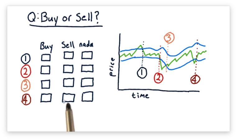
Buy or Sell Quiz Solution
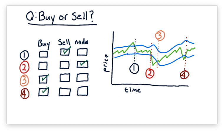
For the first event, we see the price crossing from the outside to the inside of the upper Bollinger Band. This event indicates that the price is moving back towards the moving average after a strong upward excursion. This is a sell signal.
For the second event, we see the price crossing from the inside to the outside of the lower Bollinger Band. This is not a signal, although it does indicate a significant excursion from the moving average.
For the third and fourth events, we see the price crossing from the outside to the inside of the lower Bollinger Band. These events indicate that the price is moving back towards the moving average after a strong downward excursion. Correspondingly, they are both buy signals.
Normalization
The technical indicators that we have discussed so far - simple moving averages, momentum, and Bollinger Bands - each have ranges of values over which they typically operate. For example, we might expect to see values between -0.5 and 0.5 for both simple moving averages and momentum, while we typically see values for Bollinger bands between -1.0 to 1.0.
If we were to plug these indicators into a machine learning algorithm, we might see the algorithm placing more importance on the Bollinger Bands because this indicator can take on values of a larger magnitude than the other indicators.
This undue overweighting of a particular factor might be even more visible if we include a fundamental indicator, like P/E ratio, which can range from 1 to 300.
The solution to this problem is normalization, which takes each of these parameters and compresses or stretches them so that they vary, on average, from -1 to 1, with a mean of 0. Effectively, normalization allows for an "apples to apples" comparison of variables that take on different ranges of values.
Normalizing values is simple. Given a set of original values, , we can calculate the normalized values, , as follows. Note that refers to the mean of , and refers to the standard deviation of .
OMSCS Notes is made with in NYC by Matt Schlenker.
Copyright © 2019-2023. All rights reserved.
privacy policy