The Capital Assets Pricing Model (CAPM)

Definition of a Portfolio

A portfolio is a weighted set of assets.

Let's suppose we have a portfolio of three different assets: Apple (AAPL), Google (GOOG), and Oracle (ORCL). Let's also assume that we have allocated 60% of the portfolio to APPL, and 20% each to GOOG and ORCL.

If we consider these allocations as a set of weights instead of percentages, we would say that our AAPL position has a weight of 0.6, while our GOOG and ORCL positions each have a weight of 0.2.

We can stipulate that the sum of the weights of each investment equals one; in other words, our portfolio allocations must add to 100%. Formally, given $n$ investments, where $w_i$ represents the weight of the investment in asset $i$,

However, not all weights need to be positive. For example, if we short GOOG, our allocation might be -0.2 instead of 0.2. We can refine the constraint above as follows.

For a given day, $t$, we can calculate the daily return of the portfolio, $r_p(t)$, as the weighted sum of the daily returns of each of the assets on day $t$.

Portfolio Return Quiz

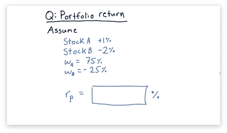
Consider a portfolio consisting of two stocks: Stock A and Stock B. 75% of the portfolio is in Stock A, and -25% of the portfolio is in Stock B; in other words, the portfolio has taken a short position in Stock B.

Assume that, today, the price of Stock A increases by 1%, while the price of Stock B decreases by 2%. What is the return on this portfolio?

Portfolio Return Quiz Solution

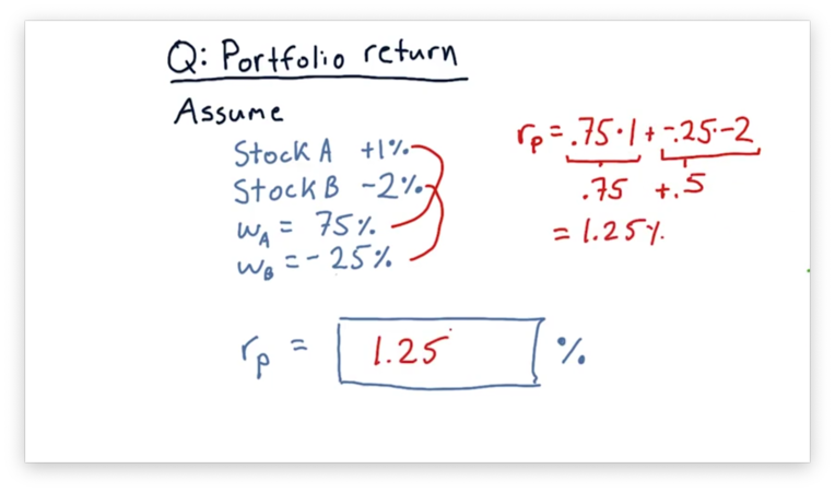
Remember the formula to calculate portfolio return.

If we plug in the weights and returns for Stock A and Stock B, we can compute a portfolio return of 1.25%.

The Market Portfolio

When someone refers to "the market", what they are usually referring to is an index that broadly covers a large set of stocks.

The best example of such an index in the United States is the S&P 500, which represents the 500 largest companies traded on stock exchanges. The value of the S&P 500 changes each day as a result of stock price fluctuations among its constituent companies.

There are similar stock market indices in other countries, such as FTA in the United Kingdom and TOPIX in Japan. Additionally, there are specialized indices that track companies only within specific industries, such as healthcare or technology.

Stock market indices are composed of many individual stocks, and the market portfolio is the combination of those stocks according to a particular weighting. Most indices are capitalization-weighted, which means that the individual weight of each stock in the portfolio is proportional to that stock's market capitalization.

Formally, given a total market capitalization $M_{total}$ of all of the stocks in the index, the weight of an individual stock with a market capitalization of $M_{individual}$ is

Some stocks have surprisingly large weightings. For example, Apple and Exxon each comprise about 5% of the S&P 500, and the 10 largest companies account for over 20% of the performance of the index. Smaller stocks may comprise only one-tenth of one percent.

The CAPM Equation

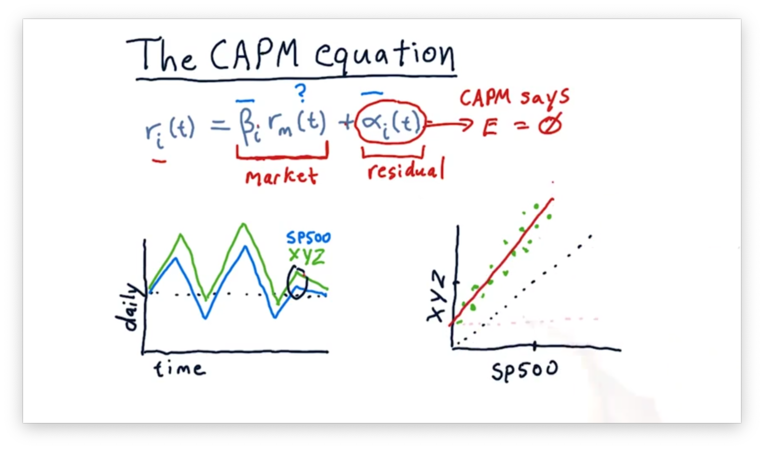
The core of the capital assets pricing model (CAPM) is captured in the following equation.

The return, $r_i$, for an individual stock, $i$, on a particular day, $t$, is equal to some stock-specific factor, $\beta_i$, times the return on the market, $r_m(t)$, plus another stock-specific factor, $\alpha_i(t)$.

Remember that when we are talking about the market, we are explicitly talking about a stock market index, such as the S&P 500, of which stock $i$ is a member.

Looking at the equation above, we see that the capital assets pricing model asserts that a significant portion of the return for a particular stock is due to the market. In other words, the movement of the market strongly affects the price of every individual stock in that market.

The $\beta$ factor encapsulates the extent to which the market affects a particular stock. Many stocks have a $\beta$ near 1, which means that when the market moves 1%, the stock also moves 1%. A larger $\beta$ indicates that a stock moves more than 1% when the market moves 1%.

If we try to compute the historical return for a particular stock based solely on the market return and $\beta$, we won't calculate the correct value. There is going to be something "left over". The $\alpha$ component of the CAPM equation captures this residual.

A crucial assertion of CAPM is that the expectation for $\alpha$ is 0. Technically, $\alpha$ is a random variable with an expected value of 0.

How do we arrive at values for $\alpha$ and $\beta$ for a particular stock? Primarily, we look at daily returns and examine how the daily returns of that stock measure against the daily returns of the market.

For example, consider the following plot of the S&P 500 daily returns alongside the daily returns for fictional stock XYZ.

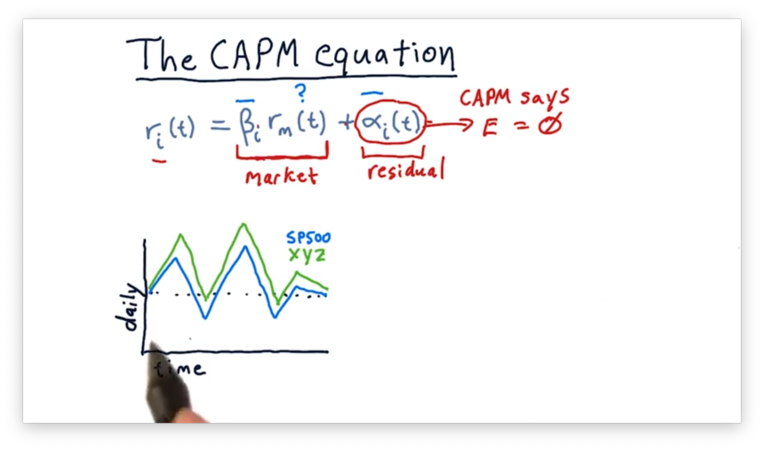
For each day, it looks like XYZ is more reactive than the S&P 500; in other words, when the S&P 500 goes up a little bit, XYZ goes up a lot. Additionally, XYZ appears to have a higher absolute return, on average, than the S&P 500.

We can create a scatterplot of the returns for XYZ against the returns for the S&P 500.

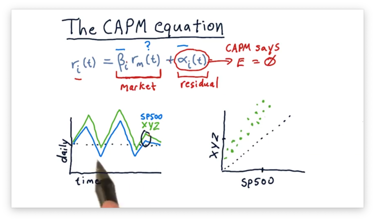
We could potentially fit the following line to this scatterplot.

Like any line, the line above can be described by two parameters: slope and y-intercept. The slope is $\beta$, and the y-intercept is $\alpha$.

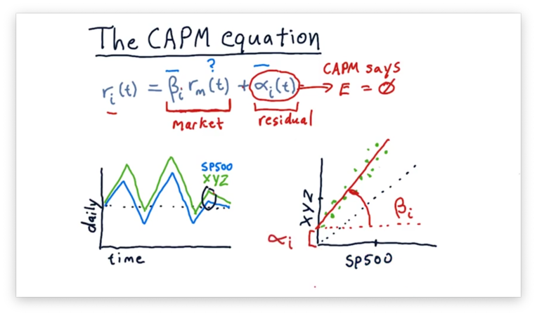
Note that this calculation of $\alpha$ and $\beta$ is after-the-fact. Just because a particular stock had a certain $\alpha$ historically doesn't mean that we can expect that value to remain in the future. Again, CAPM says that we should expect $\alpha$ to be zero; in reality, though, $\alpha$ is not always zero.

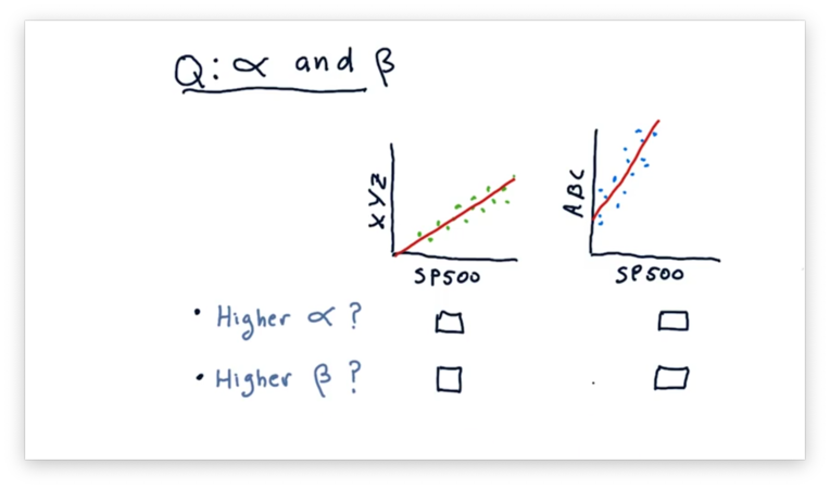
Compare Alpha and Beta Quiz

Consider the following two scatterplots. The plot on the left shows the daily returns of a fictional stock XYZ against the daily returns of the S&P 500. The plot on the right shows the daily returns of a fictional stock ABC against the daily returns of the S&P 500.

Given these two plots, which asset has a higher $\alpha$ and which has a higher $\beta$?

Compare Alpha and Beta Quiz Solution

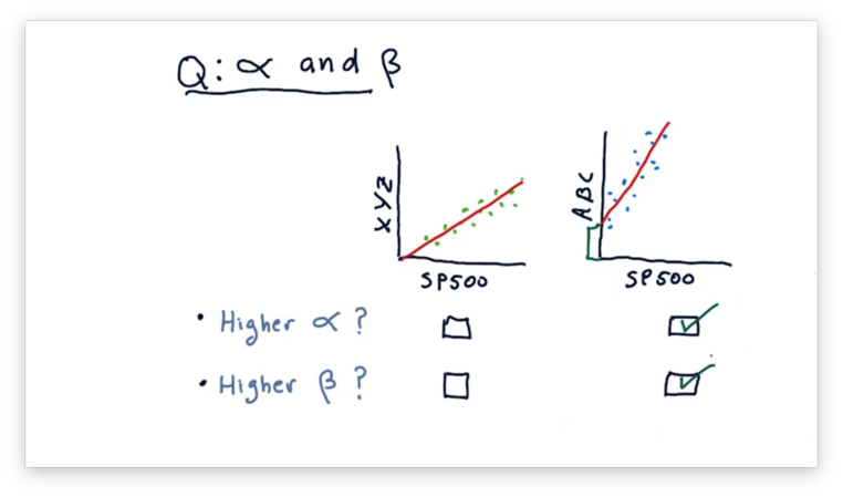
Recall that $\beta$ is the slope of the fit line, and $\alpha$ is the y-intercept of the fit line. We can tell from the plots that ABC has both a higher $\alpha$ and a higher $\beta$.

CAPM vs. Active Management

You may have heard about the debate between passive investing versus active investing. Passive investing advises investors to buy an index portfolio - for example, an ETF like SPY that tracks the S&P 500 - and hold it and let it grow. Active investing, on the other hand, is all about picking individual stocks.

Let's consider active and passive investing with regard to the CAPM equation, listed below.

Both active managers and passive managers agree with the first part of this equation; in other words, they agree that how a stock moves each day is most significantly influenced by the market, and the amount that it moves can be captured by $\beta$.

However, they disagree concerning the treatment of the $\alpha$ factor. Remember that CAPM says two essential things about $\alpha$: it's random, and it's expected value is zero. Passive investors agree with CAPM.

Active managers, on the other hand, believe that $\alpha$ is neither random nor centered around zero. They think that they can examine stocks and predict which are going to rise or fall relative to the market. They might not be exactly right on every single pick, but they believe that, on average, they are better than random and better than zero.

If you believe what active managers say, you might consider leveraging historical information as well as machine learning to find stocks that have a positive or negative $\alpha$. From there, you might be able to select a basket of stocks that can outperform the market.

If you believe CAPM, then you should be a passive investor.

CAPM for Portfolios

Suppose now that instead of looking at just one stock, we want to consider an entire portfolio. Recall that for a particular stock, $i$, it's return, $r_i(t)$, on an particular day, $t$, is equal to

To compute the return for the entire portfolio, $r_p(t)$, we compute the return for each stock, $i$, multiplied by the weight, $w_i$, of that stock in the portfolio, and sum over all the stocks in the portfolio.

We can calculate the $\beta$ for the overall portfolio, $\beta_p$, as the weighted sum of the individual $\beta$ values for each stock.

We can simplify the equation for $r_p(t)$ by plugging in $\beta_p$.

Notice that we also have an $\alpha_p(t)$ term, which is ostensibly derived as a weighted sum of the individual $\alpha_i(t)$ terms. However, since CAPM tells us that the expected value of $\alpha$ is zero, we don't need to compute $\alpha_p$ directly; instead, we can estimate it.

An active portfolio manager doesn't believe that $\alpha$ is a random variable centered at zero. As a result, they incorporate the weighted sum of individual stock $\alpha$ values into the $r_p(t)$ calculation.

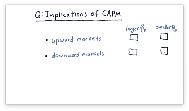
Implications of CAPM Quiz

If we are in an upward market, do we want a portfolio with a larger $\beta_p$ or a smaller $\beta_p$? How about if we are in a downward market?

Implications of CAPM Quiz Solution

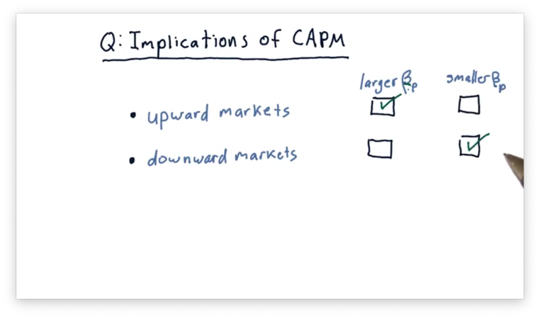
In upward markets, we want a portfolio with a larger $\beta_p$. For example, a portfolio with a $\beta_p$ greater than one rises even higher than the market, while a portfolio with a $\beta_p$ smaller than one won't be able to take full advantage of market performance.

In downward markets, we want the opposite: a smaller $\beta$. Indeed, a portfolio with a smaller $\beta_p$ falls less sharply in a downward market, while a portfolio with a larger $\beta_p$ crashes hard.

Implications of CAPM

Remember that CAPM dictates that the return of a portfolio, $r_p(t)$ depends on three things: the $\beta_p$ and $\alpha_p(t)$ of the portfolio, and the market return, $r_m(t)$.

The first point to remember is that CAPM says that $\alpha$ is a random variable with an expected value of zero. This assertion excludes smart $\alpha$ selection from our toolbox of ways to make money.

The only way we can beat the market now is by cleverly choosing $\beta$. When the market is going up, we want to invest in a portfolio with a large $\beta$. When the market is going down, we want to invest in a portfolio with a small, even negative, $\beta$.

Unfortunately, the efficient markets hypothesis - which we are going to cover soon - essentially says that you can't predict the market. As a result, the strategy of switching into portfolios with optimal $\beta$ values based on expected market performance falls flat.

If we believe CAPM, then we must concede that we cannot beat the market. Professor Balch does not believe CAPM.

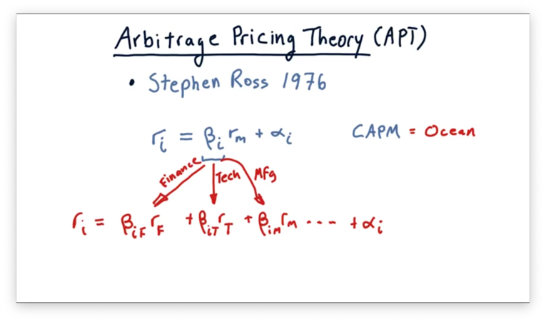
Arbitrage Pricing Theory

The classical value of $\beta$ relates the performance of a stock to the performance of the entire stock market. However, researchers realized that, since a particular stock might have exposure to multiple sectors of the market, perhaps it ought to have a $\beta$ value relating its performance to that of each sector. This is known as arbitrage pricing theory (APT).

For example, a particular stock, $i$, might have exposure to the financial sector, $F$, so we could compute the component of return for $i$ due to $F$ as the product of $\beta_{iF}$ and the return $r_F$ for $F$ for that day.

We can continue this process, computing an individual $\beta$ for each sector that impacts the stock. By breaking out the overall $\beta$ into these sector components, we can get a more accurate forecast of returns.