Working with Multiple Stocks

Pandas DataFrame Recap

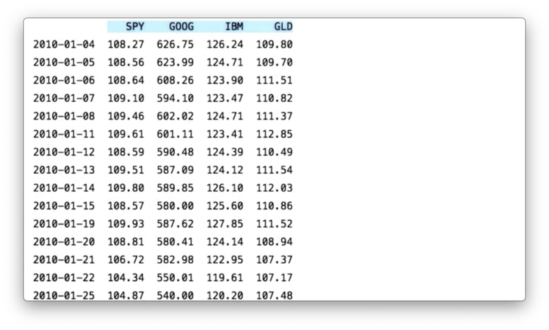
To recap, here is an illustration diagramming the structure and content of a pandas DataFrame.

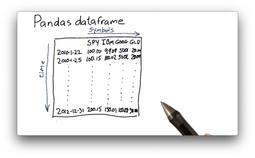
The DataFrame has columns, one for each symbol, and rows, one for each date. Each cell has a value; in this case, it is the closing price of the security represented by the symbol on the corresponding date.

Problems to Solve

To build out a DataFrame like the one pictured above, we need to consider a few things first.

For example, you might remember that our CSV file from a previous lecture contains data from 2000 through 2015. Since the DataFrame we want to build contains data from only 2010 to 2012, we need to figure out how to read in data from specific date ranges.

This new DataFrame contains information about multiple equities, whereas previous DataFrames only covered a single equity. We need to learn how to read in data for multiple stocks.

Additionally, we need a mechanism by which we can align dates. For example, if SPY traded on some days, and IBM traded on other days, we need to be able to create a DataFrame that aligns the closing prices correctly.

Finally, we need to undo the problem we discovered in the CSV from the last lecture; specifically, the dates were presented in reverse order. We need to build our DataFrame such that the chronology is as we expect: from past to present.

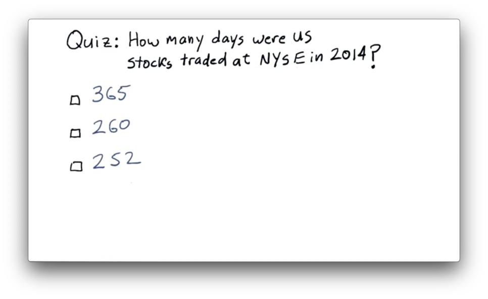
NYSE Trading Days Quiz

NYSE Trading Days Quiz Solution

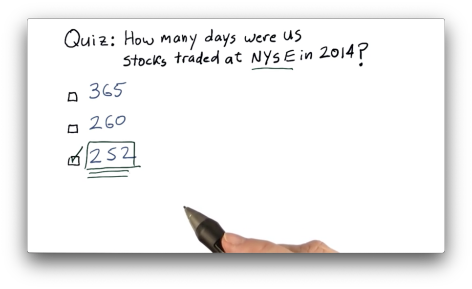
See breakdown here (for 2018 and 2019).

Building a DataFrame

We can start constructing our DataFrame by first building an empty DataFrame df, which we index by the dates that we want to consider.

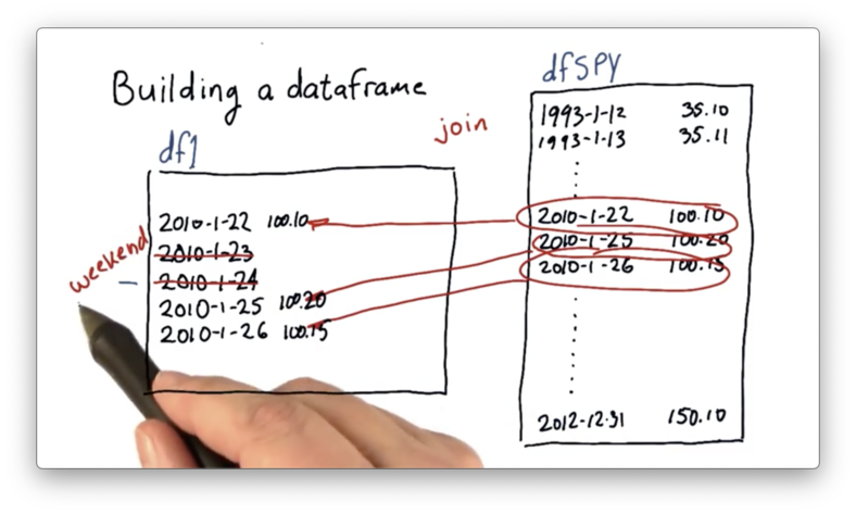
Since our goal is to load df with a column for SPY, IBM, GOOG, and GLD, we begin by reading in SPY data into a DataFrame dfSPY.

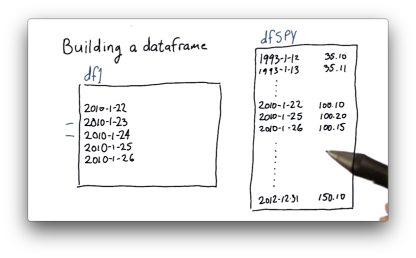
When we compare df1 and dfSPY, we notice two interesting things.

First, there are many more dates in dfSPY than there are in the target df. dfSPY contains all of the data for SPY, and we need a way to retrieve data from only the dates we are considering.

Second, there are dates present in df that are not present in dfSPY. When we constructed our index, we didn't skip weekends or holidays. Obviously, SPY did not trade on those dates since the market was not open. We will need to deal with this alignment issue.

Joining DataFrames

We now need to combine df and dfSPY into a single DataFrame. Thankfully, pandas has several different strategies for doing just that. We are going to look at an operation called a join.

There are a few different types of joins, and the names may sound familiar if you have ever taken a databases course. The type of join that we are interested in retains only those rows that have dates present in both df and dfSPY. Formally, this is known as an inner join.

Not only does the inner join eliminate the weekends and holidays originally present in df, but it also drops the dates in dfSPY that fall outside of the desired date range.

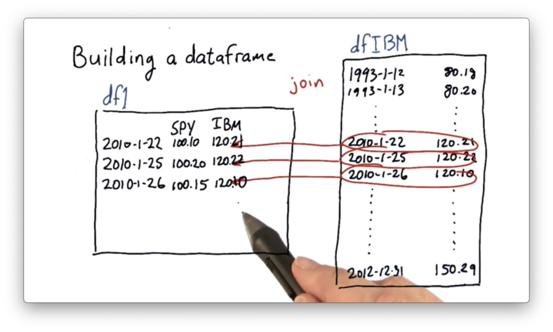
After we have joined df and dfSPY, we can repeat the procedure for the other equities - IBM, GOOG, and GLD - by performing additional joins.

Creating an Empty DataFrame

Before we start joining in our stock data, we first need to create our empty DataFrame using pandas.

We can create a date range dates that will serve as the index of our DataFrame with the following code:

start_date = '2010-01-22'
end_date = '2010-01-26'

dates = pd.date_range(start_date, end_date)

If we print dates, we see the following.

Note that dates is not a list of strings, but rather a series of DatetimeIndex objects.

We can retrieve the first object from dates by calling dates[0], which looks like the following if we print it.

The "00:00:00" represents the default timestamp, midnight, for a DateTimeIndex object. The index for our DataFrame only concerns dates, so we can effectively ignore this timestamp.

We can now create a DataFrame df that uses dates as its index with the following code:

df = pd.DataFrame(index=dates)

If we print df, we see the following.

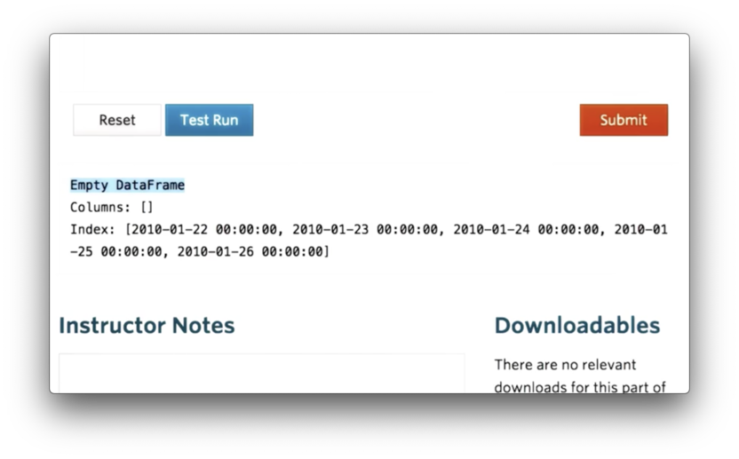
We can see that df is an empty DataFrame, with no columns, that uses dates as its index.

Documentation

• pandas.date_range
• pandas.DataFrame

Join SPY Data

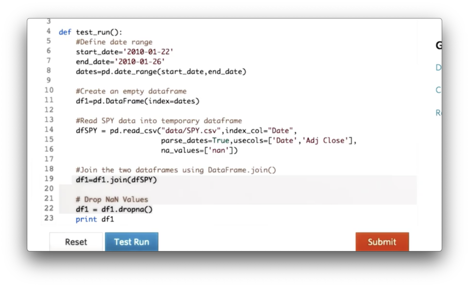
With df in place, we can now read SPY data into a temporary DataFrame, dfSPY, with the following code:

dfSPY = pd.read_csv('data/SPY.csv')

We can attempt to join the two DataFrames with the following code:

df = df.join(dfSPY)

The default join is a left join, which means the following. First, all of the rows in df are retained. Second, all of the rows in dfSPY whose index values are not present in the index of df are dropped. Third, all of the rows in df whose index values are not present in the index of dfSPY are filled with NaN values.

If we print the resulting DataFrame, relabelled as df, we see the following.

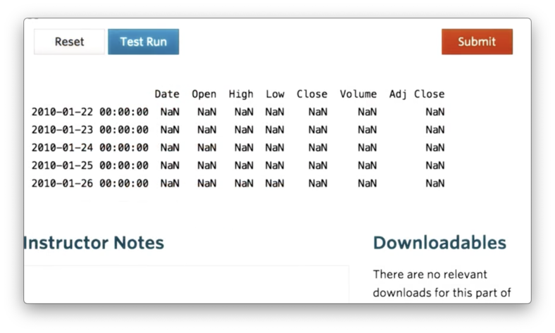
None of the values from dfSPY appear in our new df. Let's print dfSPY to debug.

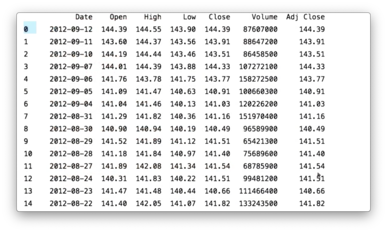
The issue here is that while df has an index of DatetimeIndex objects, dfSPY has a simple, numeric index.

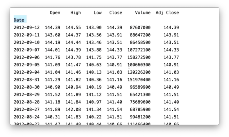
We can rectify this by telling pandas that the Date column of the SPY CSV should be used as the index column and that the values in this column should be interpreted as dates. We accomplish this with the following code:

dfSPY = pd.read_csv('data/SPY.csv', index_col="Date", parse_dates=True)

If we print dfSPY now, we see the following, correct DataFrame.

Since we only care about the adjusted close and the date columns, we can construct dfSPY to only include those columns using the usecols parameter.

Additionally, we can replace textual values representing null or absent values with proper NaNs using the na_values parameter. In the SPY CSV, NaN is represented by the string "nan".

The full initialization of dfSPY is demonstrated by the following code:

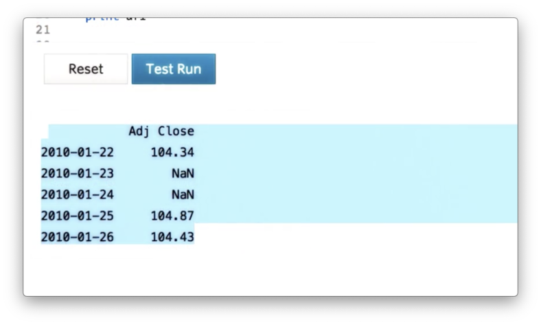
dfSPY = pd.read_csv('data/SPY.csv', index_col="Date", parse_dates=True, usecols=["Date", "Adj Close"], na_values=['nan'])

If we again print df, the result of the join, we see the following DataFrame.

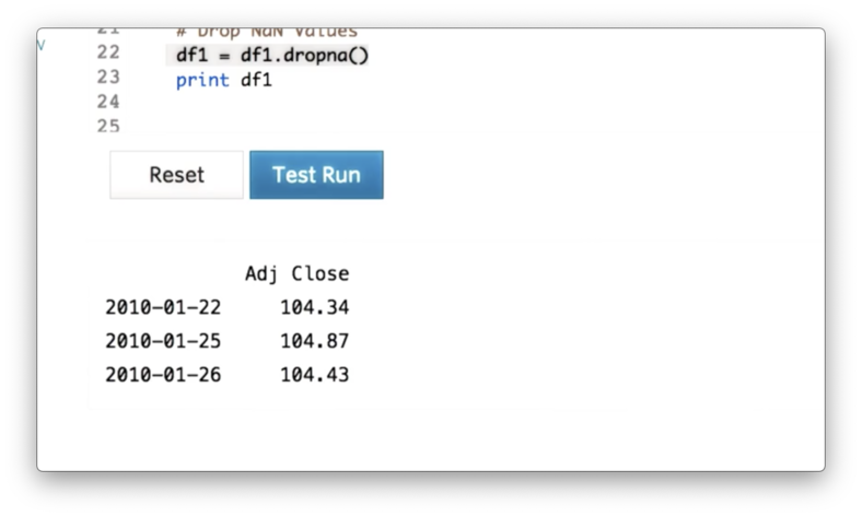
Finally, we can drop weekends and holidays - where adjusted close is NaN - using the following code:

df = df.dropna()

If we print out df, we see the following, correct DataFrame.

Documentation

• pandas.read_csv
• pandas.DataFrame.join
• pandas.DataFrame.dropna

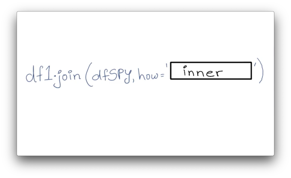
Types of Joins Quiz

We can avoid having to explicitly call dropna on line 22 by passing a certain value for the 'how' parameter of the join call on line 19.

What is the value of that parameter?

Types of Joins Quiz Solution

Documentation

• pandas.DataFrame.join

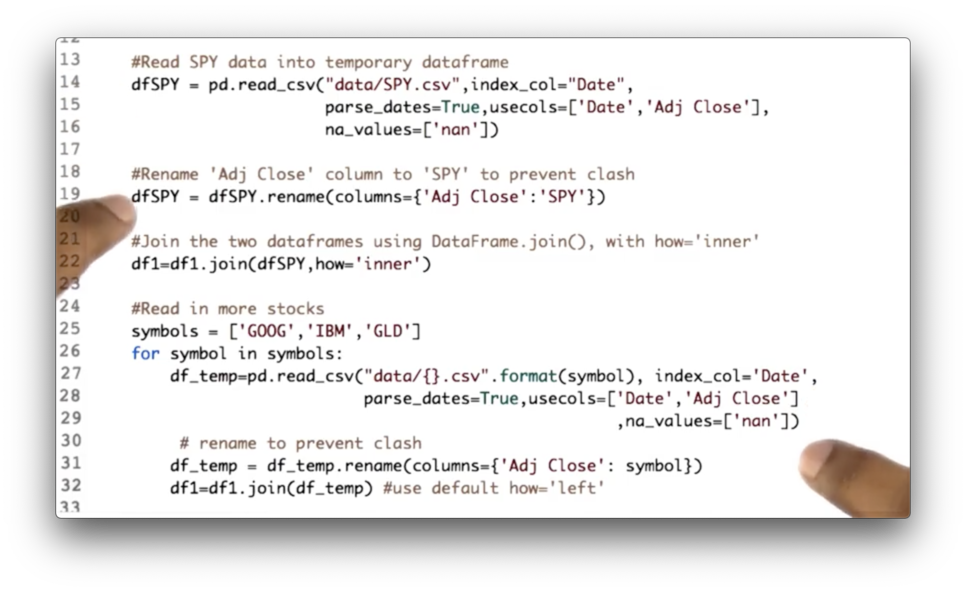
Read in More Stocks

We want to read in data about three more stocks - GOOG, IBM, and GLD - and create our complete DataFrame. We can iterate over the stock symbols, create temporary DataFrames, and join them to df with the following code:

for symbol in symbols:
	df_temp = pd.read_csv('data/{}.csv'.format(symbol), index_col="Date", parse_dates=True, usecols=["Date", "Adj Close"], na_values=['nan'])

	df = df.join(df_temp)

However, when we try to print df, we see an error.

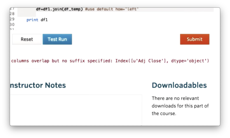
The issue here is that we have multiple DataFrames that each has a column name "Adj Close". Pandas complains that it does not know how to resolve the overlap when joining DataFrames with identical column names. In other words, column names must be unique.

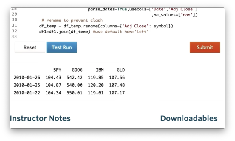
Instead of having four columns with the same name, we'd like to name each column after the symbol whose data it contains. We can accomplish that with the following code:

df_temp = df_temp.rename(columns={'Adj Close': symbol})

If we print df now, we see the following, correct output.

Documentation

• pandas.DataFrame.rename

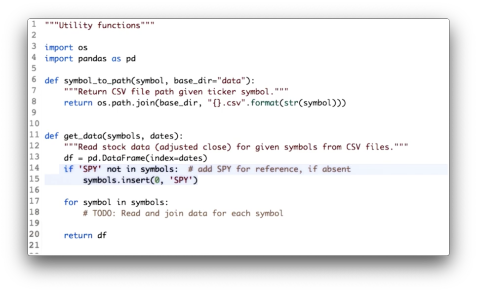
Utility Functions for Reading Data Quiz

If we look at the code we have written so far, we see some duplication.

Your task is to consolidate this code into one location: the utility function get_data.

Utility Functions for Reading Data Quiz Solution

We have consolidated both the DataFrame initialization code and the joining code.

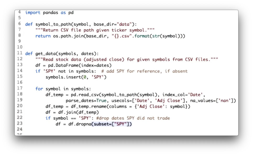
Additionally, since we are using SPY as our baseline, we drop all rows from df where SPY has not traded - that is, where the SPY column has NaN values - with the following code:

df = df.dropna(subset=["SPY"])

Documentation

• pandas.DataFrame.dropna

Obtaining a Slice of Data

Here is our complete DataFrame, containing data from 2010 to 2012 for SPY, IBM, GOOG, and GLD.

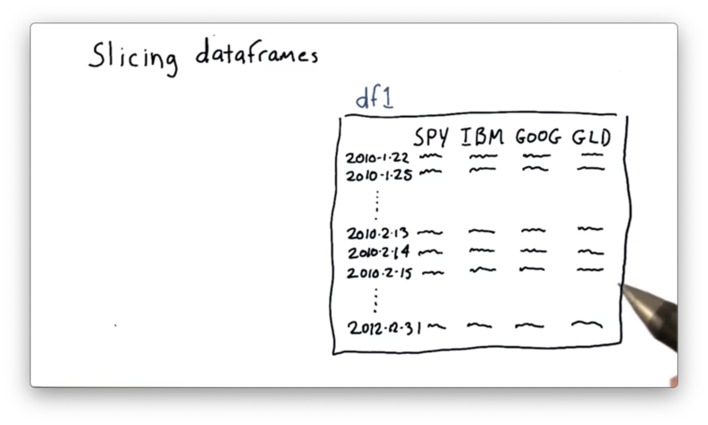
Suppose we want to focus on a subset, or a slice or this data; for instance, we might be interested in just values of GOOG and GLD for 2/13/10 through 2/15/10.

Pandas exposes a syntax for creating such a slice. Given a DataFrame df, we can retrieve the data for all columns between these two dates with the following expression:

df['2010-2-13':'2010-2-15']

We can further scope this slice to include information about only GOOG and GLD with the following expression:

df['2010-2-13':'2010-2-15', ['GOOG', 'GLD']]

Note that neither the rows nor the columns that we slice must be contiguous in df. The following slice of nonadjacent columns IBM and GLD is just as valid as our original slice:

df['2010-2-13':'2010-2-15', ['IBM', 'GLD']]

Documentation

• Slicing ranges

More Slicing

Our original DataFrame only contained data for four days. We can read in data for the whole year of 2010 by changing the dates of the DatetimeIndex object we built at the beginning of this lesson:

start_date = '2010-01-01'
end_date = '2010-12-31'

dates = pd.date_range(start_date, end_date)

If we rebuild df with this new index and print it out, we see the following.

Pandas offers several different options for slicing DataFrames.

Row slicing gives us the requested rows and all of the columns. This type of slicing might be useful when you want to compare the movement of all the stocks over a subset of time.

If we want to retrieve data for all of the symbols during January, for example, we can use the following code:

df.ix['2010-01-01':'2010-01-31']

Note that this code is equivalent to the following:

df['2010-01-01':'2010-01-31']

However, the former is considered to be more pythonic.

aside: it's not. The ix method has since been deprecated, and users should use either the loc or iloc methods.

Column slicing returns all of the rows for a given column or columns, and is helpful when we want to view just the movement of a subset of stocks over the entire date range.

The following code shows the syntax for retrieving information for just GOOG, as well as for both IBM and GLD.

df['GOOG']
df[['IBM', 'GLD']] # Note the second pair of []

Finally, we can slice through both rows and columns. For example, we can select information about just SPY and IBM, for just the dates between March 10th and March 15th:

df.ix['2010-03-10':'2010-03-15', ['SPY', 'IBM']]

Documentation

• pandas.DataFrame.ix - DEPRECATED
• pandas.DataFrame.loc
• pandas.DataFrame.iloc

Problems with Plotting

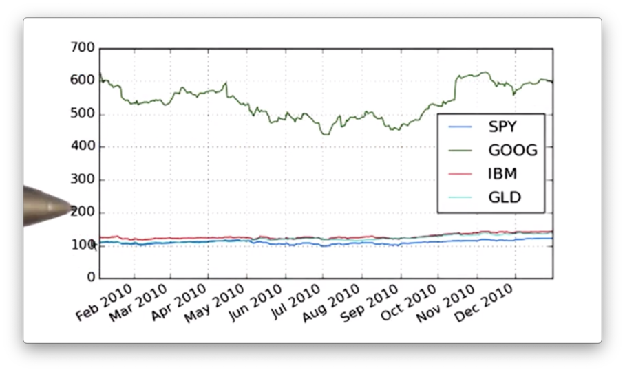
It's pretty easy to generate a good-looking plot from a DataFrame; in fact, we merely have to call the plot method.

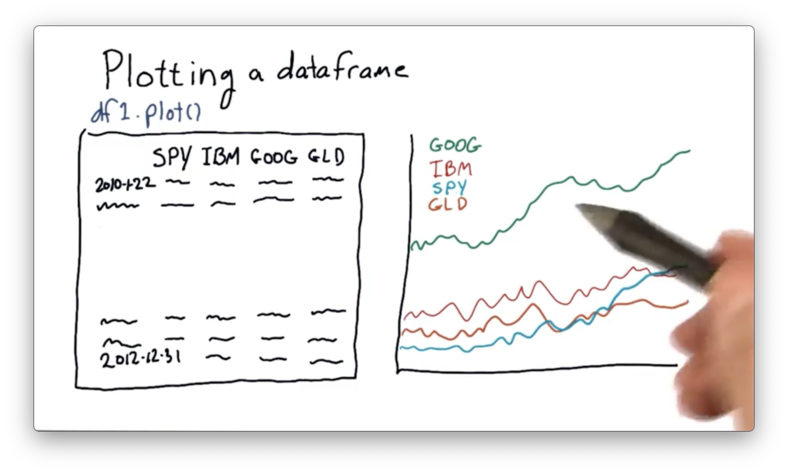
One feature that we can immediately notice about this plot is that GOOG is priced quite higher than the other stocks. It's often the case that different stocks are priced at significantly different levels.

As a result, it can be hard to compare these stocks objectively. We'd like to adjust the absolute prices so that they all start from a single point - such as 1.0 - and move from there.

If we can normalize the stock prices in this manner, we can more easily compare them on an "apples to apples" basis.

Documentation

• Plotting

How to Plot on "Equal Footing" Quiz

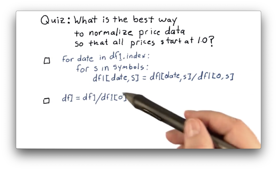
How to Plot on "Equal Footing" Quiz Solution

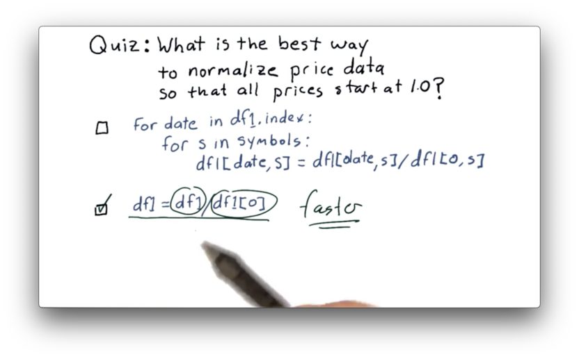
While both of these are technically correct, the second approach leverages vectorization which is must faster than the iterative approach. Read more about vectorization here.

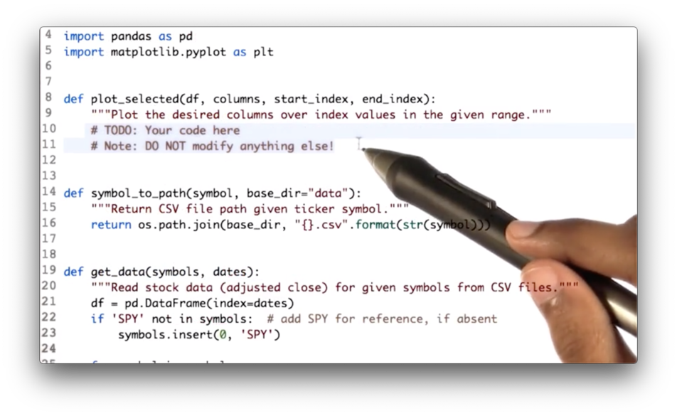
Plotting Multiple Stocks

To plot our data, we first need to import matplotlib. We can then define a plot_data function that receives a DataFrame df and calls plot on it.

import matplotlib.pyplot as plt

def plot_data(df):
    df.plot()
    plt.show() 

If we run this function, we see the following graph.

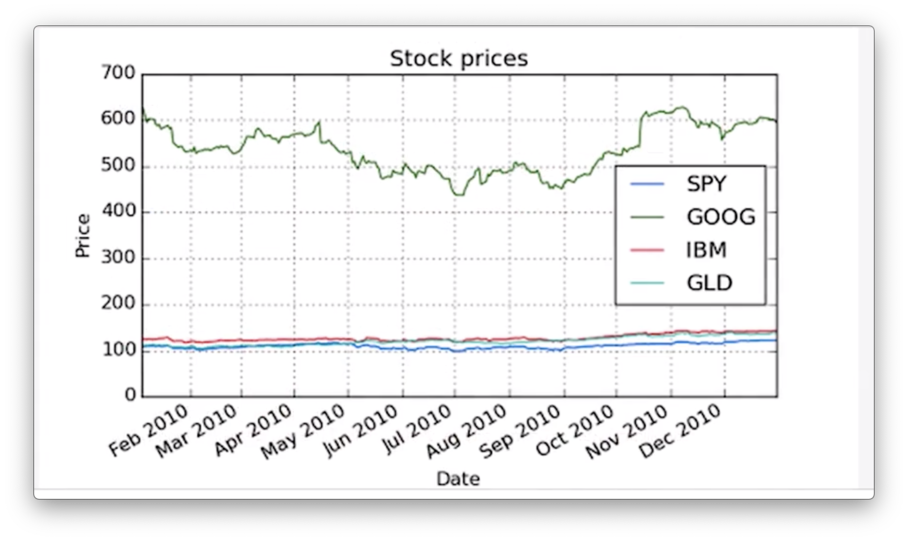
We need to add more information to our graph, such as a title as well as x- and y-axis labels. Additionally, we can change the font-size of the text to improve readability. We can adjust the title and the font-size with the following code:

def plot_data(df, title="Stock Prices"):
    df.plot(title=title, fontsize=2)
    plt.show()

To generate axis labels, we need to call the set_xlabel and set_ylabel methods on the object that the plot method returns.

def plot_data(df, title="Stock Prices"):
    ax = df.plot(title=title) # ax for axis
    ax.set_xlabel("Date")
    ax.set_ylabel("Price")
    
    plt.show()

If we run this function now, we see a more informative graph.

Documentation

• Plotting
• matplotlib.axes.Axes.set_xlabel
• matplotlib.axes.Axes.set_ylabel

Slice and Plot Two Stocks Quiz

Your task is to write code that first slices df along the rows bounded by start_index and end_index and across columns, and then passes the slice to the plot_selected method.

Slice and Plot Two Stocks Quiz Solution

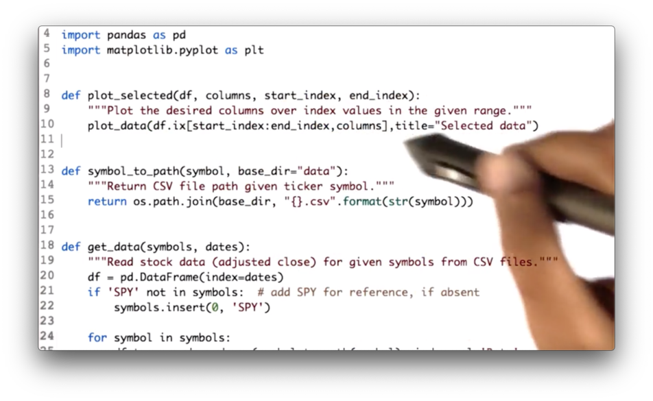
We can create our slice using the following code, which we then pass to the plot_data method:

df.ix[start_index:end_index, columns]

Documentation

• pandas.DataFrame.ix - DEPRECATED
• pandas.DataFrame.loc
• pandas.DataFrame.iloc

Normalizing

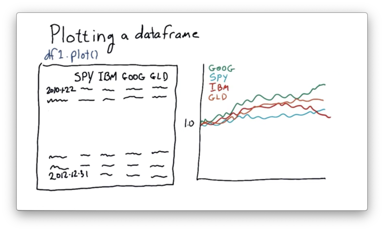
Let's take another look at the plot we have created.

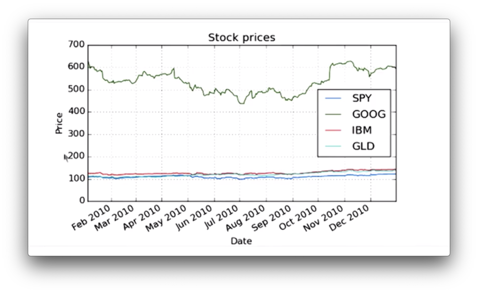
Here we see the absolute price movement of each stock. What we are more interested in, however, is the price movement of each stock relative to its starting price.

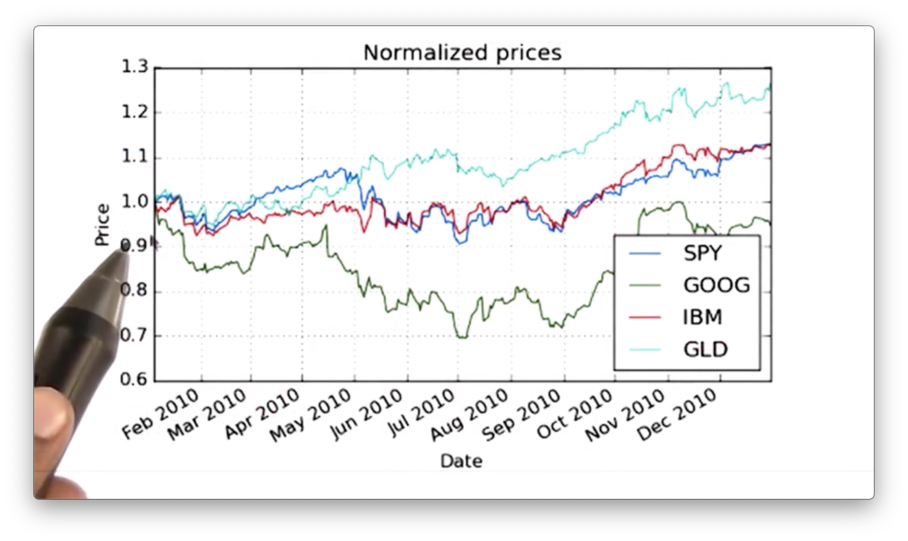
To create a plot that shows this relative movement, we first need to normalize the prices of each stock. We do this by dividing the values of each column by their price on day one. This ensures that each stock starts at 1.0.

We can create a normalize_data method that normalizes the data in a DataFrame df:

def normalize_data(df):
    return df / df.ix[0, :]

If we graph our normalized DataFrame, we see the following graph. Notice that all the stocks start at 1.0 and move from there.