Portfolio Optimization and the Efficient Frontier

Overview

Suppose you have a set of stocks that you have determined are valuable investments. How much of your portfolio should you invest in each? In this lesson, we are going to look at the following portfolio optimization problem: given a set of equities and a target return, find an allocation to each equity that minimizes risk.

What is Risk

If we are going to find a portfolio - an allocation of assets to different stocks - that minimizes risk, we have to consider first: what is risk?

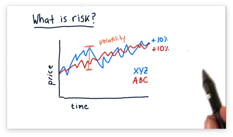
The standard measurement for risk is volatility, the standard deviation of historical daily returns.

Let's consider two stocks, XYZ and ABC, that have both gone up 10%. Since the price movements for XYZ have been significantly more volatile than those for ABC, we consider XYZ a riskier investment.

Visualizing Return Vs. Risk

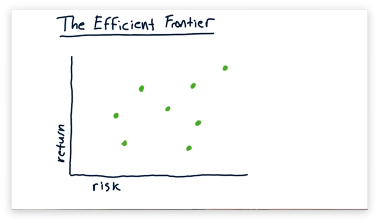
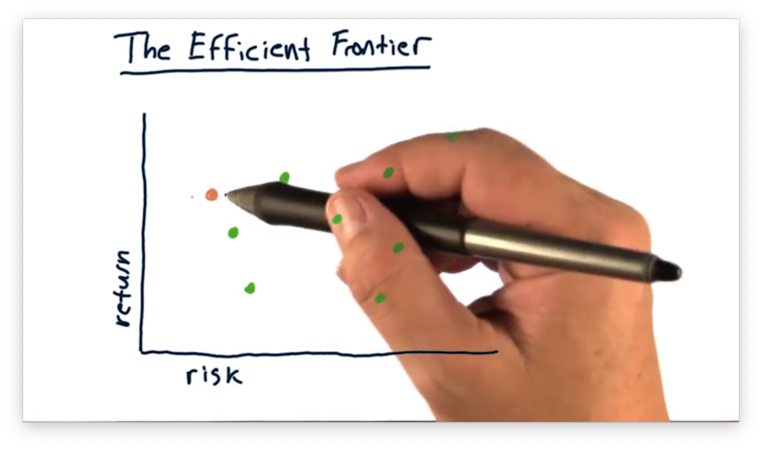
We often want to consider multiple stocks together and evaluate their relative risk versus their relative return. One way we can visualize this relationship is to plot each stock on a scatterplot, where the x-axis measures risk, and the y-axis measures return.

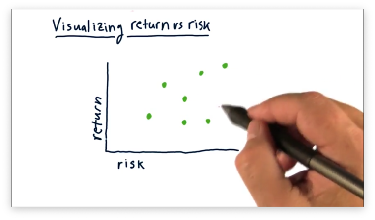
With a plot like this, we can easily compare stocks along these two dimensions. For example, stocks situated closer to both axes have relatively lower risk and return than those further away.

We build a portfolio by combining multiple assets, like the ones above, and weighting each asset by a particular weight that represents its allocation within the portfolio.

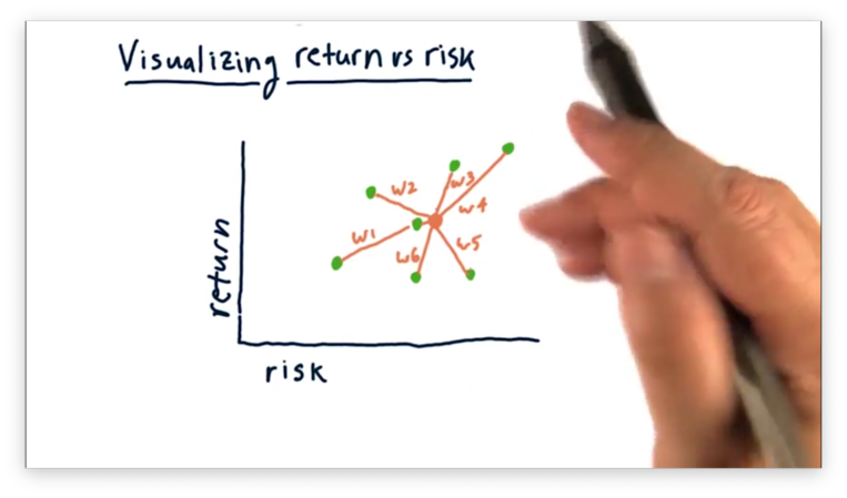
Notice that the risk and return of the aggregate portfolio is some weighted average of the constituent stocks. In other words, the portfolio risk is between that of the riskiest and safest stocks, and the portfolio return is between that of the highest- and lowest-returning stocks.

Building a Portfolio Quiz

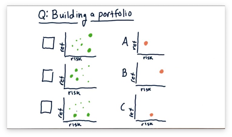
Let's consider the three following portfolios.

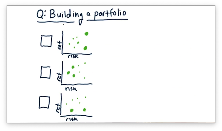
Each green dot represents an asset held in the portfolio, and the size of the dot represents the weight of that asset.

If we were to aggregate the risk and return of the individual stocks into one value, which of the following plots - in orange below - would match which portfolio?

Building a Portfolio Quiz Solution

The first portfolio emphasizes two high-risk stocks: one with low return and one with high return. Of the three plots, B looks best-aligned for this allocation.

The second portfolio emphasizes three low-risk stocks with an aggregate middle-of-the-road return. Of the three plots, A looks best-aligned for this allocation.

Finally, the third portfolio emphasizes two low-return stocks: one with low risk and one with high risk. Of the three plots, C looks best-aligned for this allocation.

Can We Do Better

For a long time, people built portfolios in this manner. They would take a collection of assets, weight them relatively equally, and created a portfolio that averaged out the individual characteristics of each asset contained within.

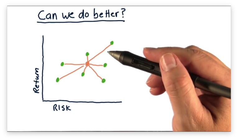
Can we do better than this "average" performance? In other words, given a collection of assets, can we derive allocations such that we create a high-return, low-risk portfolio?

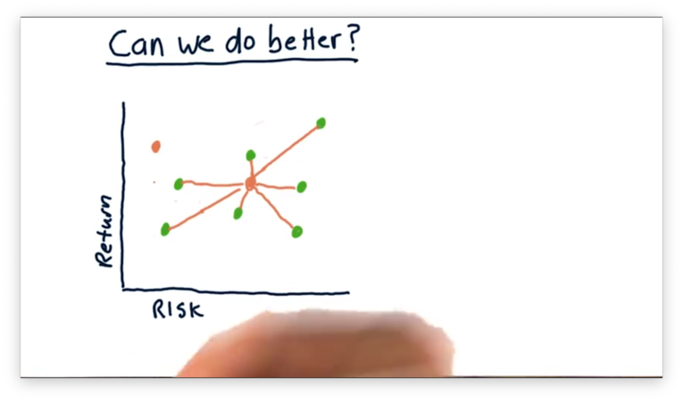
Harry Markowitz, who later won the Nobel Prize for his insight, showed that we could do better. What he uncovered, and what people had been overlooking, was the relationship between stocks in terms of covariance.

The performance of a portfolio, especially in terms of risk, is not merely a weighted average of the various performances but must take into account how each asset interacts with one another on a daily basis.

As a result, there exists an allocation for a collection of assets, which leverages these interactions, such that the resulting portfolio achieves a higher risk-adjusted return than any of the individual assets.

Up until the time of Harry Markowitz's discovery, many viewed bonds as the asset with the lowest risk. Markowitz showed that a blend of stocks and bonds is actually less risky than a portfolio containing either asset exclusively.

Why Covariance Matters

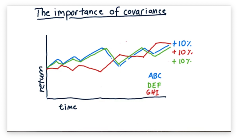
To illustrate the importance of covariance, let's look at a few different stocks. We see the performance of ABC and GHI over time in the plot below. While both stocks have returned 10%, notice that GHI tends to "zig" when ABC "zags".

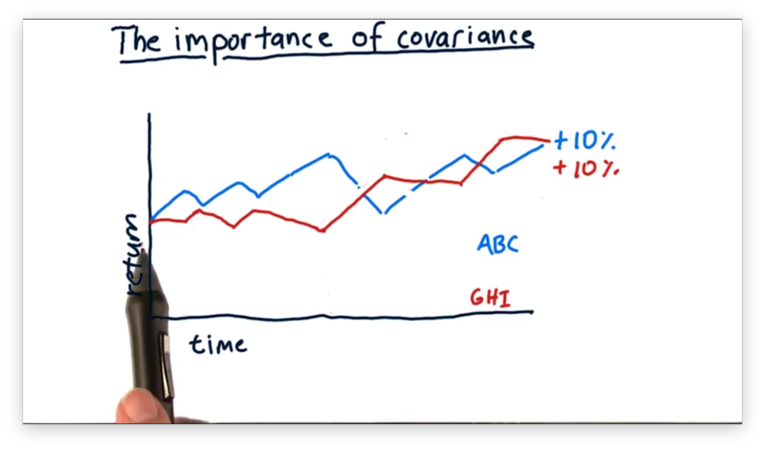
Consider also DEF, which moves practically in lockstep with ABC.

What is the best portfolio we can build by combining ABC, DEF, and GHI? To answer this question, let's think about the covariance between the assets.

ABC and DEF move very similarly, and if we were to measure the covariance of the daily returns between these two stocks, we might see a value of 0.9.

If we were to measure the covariance of daily returns between ABC and GHI, we would come up with a negative number; in other words, when ABC goes up, GHI tends to go down. We might expect a covariance value of -0.9 for these two assets.

Let's first consider a portfolio that is 50% ABC and 50% DEF. Since both assets move very similarly, a portfolio containing both of those assets would follow a very similar path.

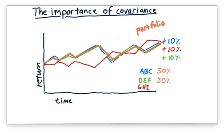
This portfolio is fine - it still returns 10% - but there is no real advantage in blending these two assets because the portfolio retains the same volatility as the individual assets.

Consider instead of portfolio with the following allocation: 25% ABC, 25% DEF, and 50% GHI. What is the effect of putting an anti-correlated asset into our portfolio?

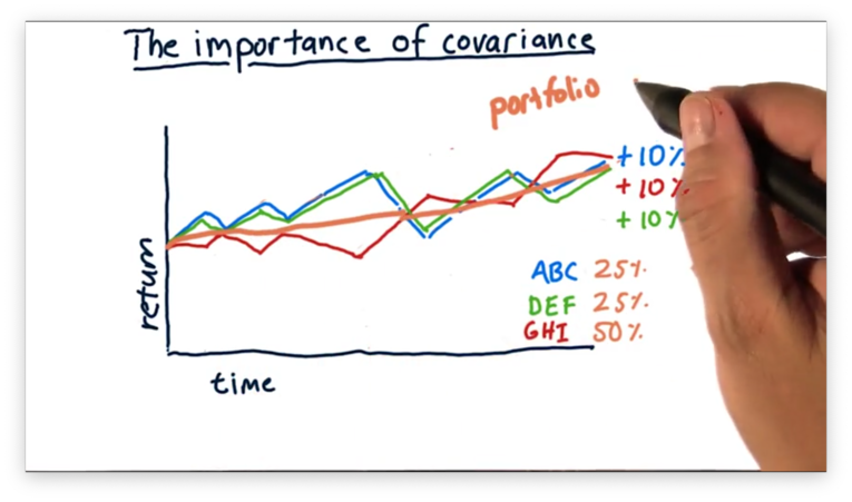
We see that this portfolio again posts 10% returns, but has much less volatility since the component stocks tend to move in opposite directions.

Thus, we have demonstrated at a high level what Markowitz proved: we can take a collection of stocks and, with a smart allocation, create a portfolio with higher - in this case, equal - return and lower risk than any component stock.

Mean Variance Optimization

When Markowitz began to consider the covariance between individual stocks, he discovered that low-risk portfolios were possible by blending together anti-correlated assets.

Out of his work grew several algorithms. Mean-variance optimization is one such algorithm, which examines the covariance between a potential set of assets to determine how a portfolio manager ought to blend them.

A mean-variance optimization algorithm takes several inputs. For each stock, we have to provide the expected return and the historical volatility of the stock. Additionally, we have to supply a covariance matrix that contains the covariance of historical returns between every pair of stocks under consideration.

Finally, we need to provide the target return we want to achieve, which can range from the return of the lowest-performing asset to that of the highest-performing asset. We can accomplish a return between the maximum and minimum values through blending.

The optimizer outputs a set of weights - one per asset - that corresponds to the allocation that each asset deserves in the portfolio. According to the optimizer, such a portfolio provides the target return but minimizes risk.

The Efficient Frontier

Consider the following assets.

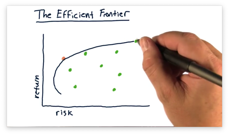
For any particular desired return, there exists an optimal - minimally risky - portfolio. For example, we can see the optimal portfolio for one value of return below.

We can plot the optimal portfolio for each value of desired return and connect the points to form a line.

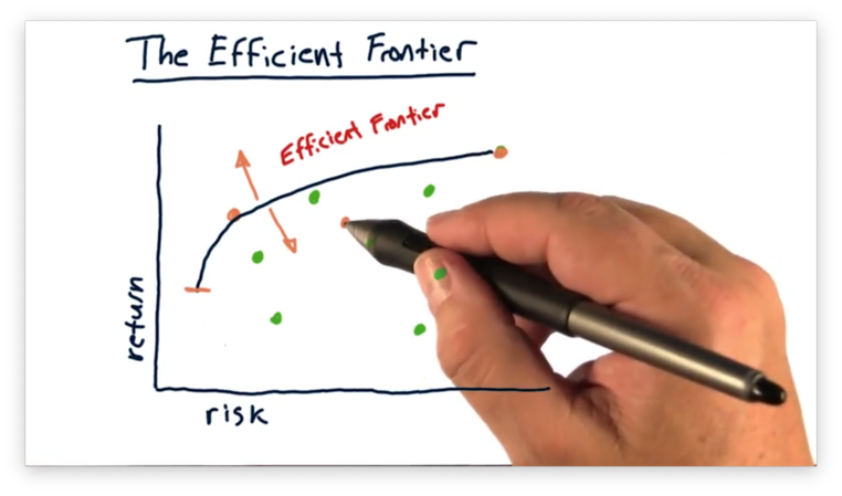
Note that, as we reduce the return, the associated risk sometimes increases. Naturally, few people want low-return, high-risk portfolios, so we often don't consider this portion of the curve.

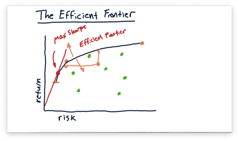
We call this curve the efficient frontier. The efficient frontier represents the ceiling for portfolio return, given a particular amount of risk. As a result, there are no portfolios "beyond" the efficient frontier, and any portfolio "behind" the frontier is insufficient in some way.

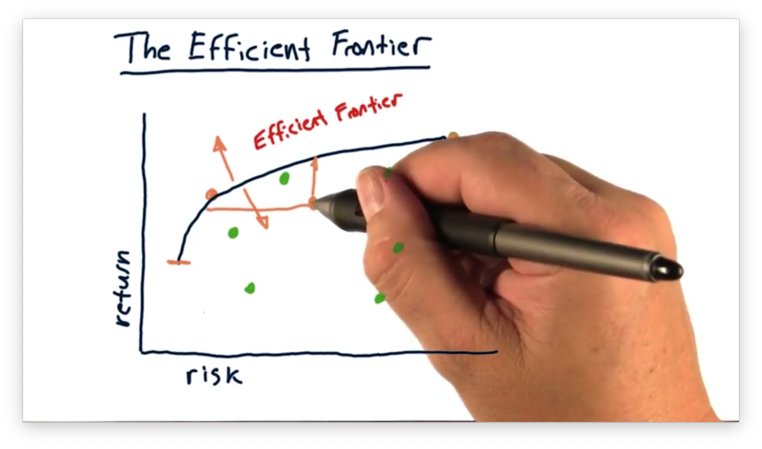
For example, consider this portfolio.

This portfolio is suboptimal; that is, for the amount of return it achieves, it assumes way too much risk. Said another way, this portfolio achieves too little return for the amount of risk it bears.

Given this level of risk and this collection of assets, there exists a portfolio that achieves a higher return. Conversely, given this level of return, there exists a portfolio that bears significantly less risk.

One last thing to note about the efficient frontier is that, if we draw a tangent line on the frontier, originating from the origin, the slope of that line represents the maximum Sharpe ratio we can achieve with this collection of assets.

The efficient frontier is primarily a theoretical device; however, some portfolio managers like to plot the frontier so that they can see where their portfolio lies relative to the assets it comprises and the efficiency it might achieve.