Reinforcement Learning

Overview

Until now, we've built models that forecast price changes and then used these models to buy or sell the stocks with the most significant predicted change. This approach ignores some important issues, such as the certainty of the prediction and when to exit a position. We are going to shift our focus now to reinforcement learning. Reinforcement learners create policies that provide specific direction on which action to take given a particular set of parameters.

The RL Problem

When we talk about reinforcement learning, we are talking about a problem, not a solution. In the same way that linear regression is one solution to the supervised regression problem, there are many algorithms that solve the reinforcement learning problem.

To demonstrate one possible algorithm, let's consider a robot interacting with the environment.

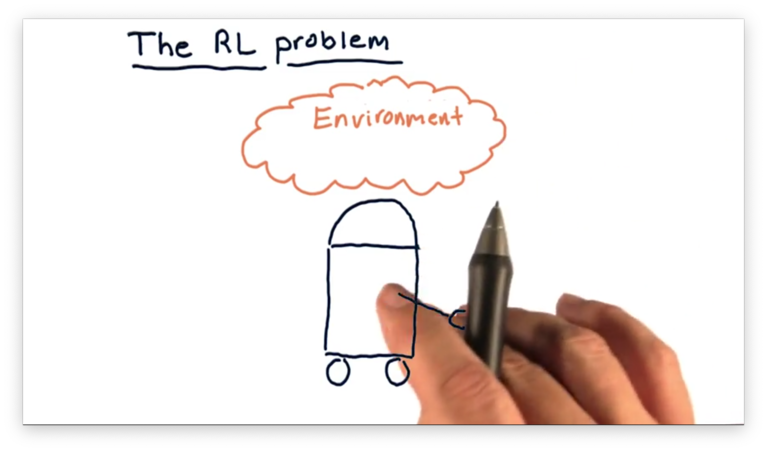
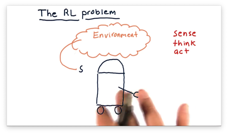
First, the robot observes the environment; more specifically, it reads in some representation of the environment. We call this representation the state, which we denote as $S$.

The robot has to process $S$ to determine what action to take and does so by consulting a policy, which we denote as $\pi$. The robot considers $S$ with regard to $\pi$ and outputs an action $a$.

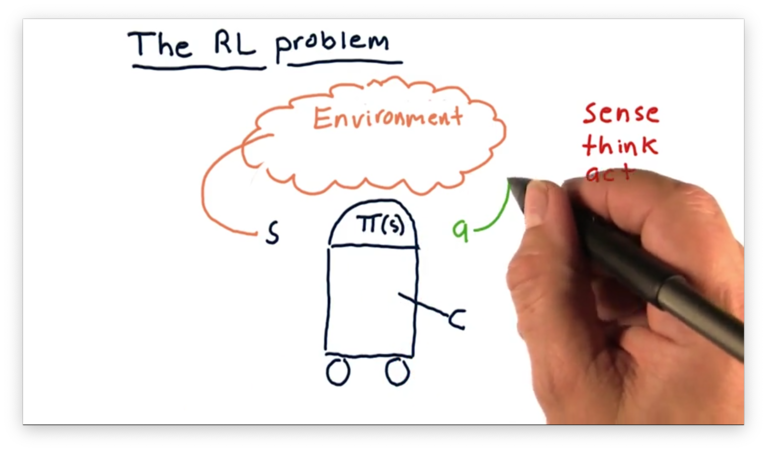
The action $a$ changes the environment in some way, and we can use a transition function, denoted as $T$, to derive a new environment from the current environment and a particular action.

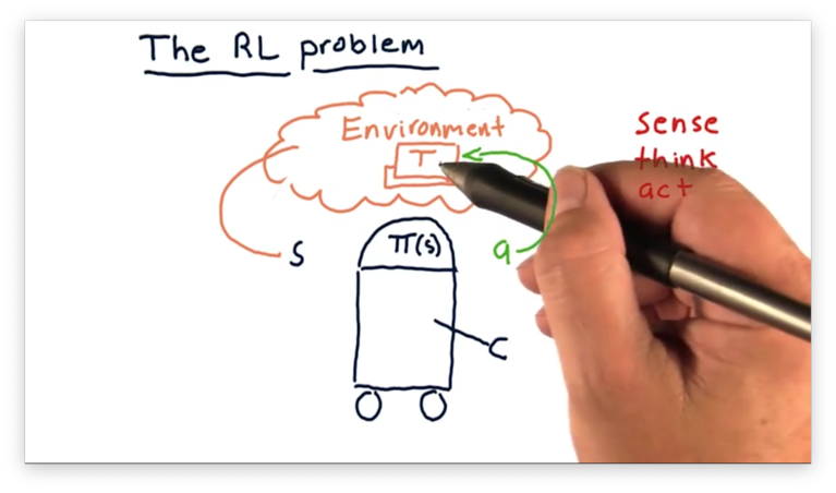
Naturally, the robot reads in the updated environment as a new $S$, against which it consults $\pi$ to generate a new $a$. We refer to this circular process as the sense, think, act cycle.

To understand how the robot arrives at the policy $\pi$, we have to consider another component of this cycle: the reward, $r$. For any action that the robot takes, in any particular state, there is an associated reward.

As an example, if a navigation robot senses a cliff ahead and chooses to accelerate, the associated reward might be very negative. If, however, the robot chooses to turn around, the reward might be very positive.

In our case, we can imagine that our robot has a little wallet where it keeps its cash. The reward for a particular action might be how much cash that action adds to the wallet. The objective of this robot is to execute actions that maximize this reward.

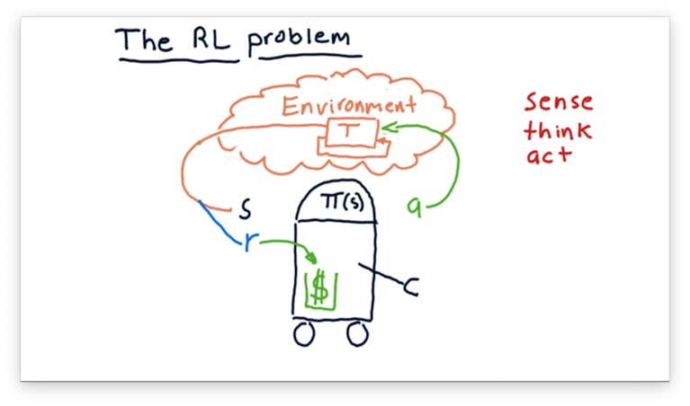
Somewhere within the robot, there is an algorithm that synthesizes information about $S$, $r$, and $a$ over time to generate $\pi$.

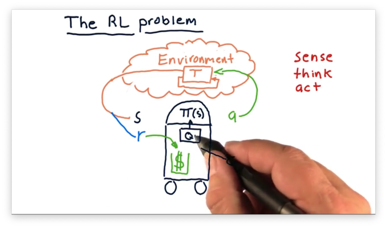
To recap, $S$ is the state of the environment that the robot "senses", and it uses a policy $\pi$ to determine which action $a$ to take. Each action comes with an associated reward $r$, and the robot tries to refine $\pi$ over time to maximize $r$.

In terms of trading, the environment is the market, and the available actions correspond to the actions that we can take in the market, such as buying, selling, or holding. $S$ corresponds to different factors about our current portfolio that we might observe, and $r$ is the return we get for making specific trades.

Trading as an RL Problem Quiz

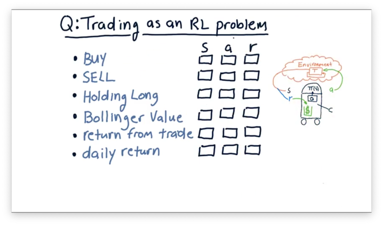
We want to use reinforcement learning algorithms to trade; to do so, we have to translate the trading problem into a reinforcement learning problem.

Consider the following items. For each item, select whether the item corresponds to a component of the external state $S$, an action $a$ we might take within the environment, or a reward $r$ that we might use to inform our policy $\pi$.

Trading as an RL Problem Quiz Solution

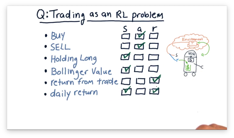
Buying and selling stock are both actions that we execute upon our environment.

Holding long and Bollinger value are both parts of the state. Holding long tells us about our position in a particular stock, and Bollinger value tells us about the current price characteristics of a stock. Both of these pieces of information might drive subsequent action.

The return from a trade is our reward. If our return is positive, so is our reward. On the other hand, a negative reward indicates that we lost money on the position. Daily return could be either a component of the state - a factor we consider before generating an action - but it could also be a reward.

Mapping Trading to RL

Let's think about how we can frame stock trading as an RL problem. In trading, our environment is the market. The state that we process considers, among other factors: market features, price information, and whether we are holding a particular stock. The actions we can execute within the environment are, generally, buy, sell, or do nothing.

In the context of buying a particular stock, we might process certain technical features - like Bollinger Bands - to determine what action to take. Suppose that we decide to buy a stock. Once we buy a stock, that holding becomes part of our state.

We have transitioned from a state of not holding to holding long through executing the buy action. We can transition from a state of holding long to not holding by executing the sell action.

Suppose the price increases, and we decide to execute a sell. The money that we made, or lost, is the reward that corresponds to the actions we took. We can use this reward and its relationship to the actions and the state to refine our policy, thus adjusting how we act in the environment.

Markov Decision Problems

Let's formalize some of the components that we have been discussing.

We have a set of states, $S$, which corresponds to all of the different states that our robot can receive as input. Additionally, we have a set of actions, $A$, which enumerates all of the potential actions we can execute within the environment.

Additionally, we have a transition function, $T$. This function takes in three arguments: a current state, $S_c$, an action, $A_i$, and a future state $S_f$. Given these three values, the transition function returns the probability that $A_i$ applied to $S_c$ brings about $S_f$.

For a particular $S_c$ and $A_i$, we are going to end up in some new state. As a result, the sum of the probabilities of state transitions from $S_c$ to some $S_f$ in $S$ for $A_i$ must equal 1.

Finally, we have the reward function $R$, which receives an action, $A_i$, and a state, $S_i$, as input and returns the reward for executing that action in that state.

A problem parameterized by these four components is known as a Markov decision process.

The problem for a reinforcement learning algorithm is to find a policy $\pi$ that maximizes reward over time. We refer to the theoretically optimal policy, which the learning algorithm may or may not find, as $\pi^*$.

There are several algorithms that we can deploy to find $\pi$ - assuming we know $T$ or $R$ - such as policy iteration and value iteration. In this class, however, we don't know $T$ or $R$ ahead of time, so we can't use either of these algorithms directly.

Unknown Transitions and Rewards

Most of the time, we don't know the transition function, $T$, or the reward function, $R$, a priori. As a result, the reinforcement learning agent has to interact with the world, observe what happens, and work with the experience it gains to build an effective policy.

Let's say our agent observed state $s_1$, took action $a_1$, which resulted in state $s^{'}_1$ and reward $r_1$. We refer to the object $(s_1, a_1, s^{'}_1, r_1)$ as an experience tuple.

The agent iterates through this sense-think-act cycle over and over again, gathering experience tuples along the way. Once we have collected a significant number of these tuples, we can use two main types of approaches to find the appropriate policy, $\pi$.

The first set of approaches is model-based reinforcement learning. In model-based reinforcement learning, we look at the experience tuples over time and build a model of $T$ and $R$ by examining the transitions statistically. For example, for each state, action pair $s_i, a_i$, we can look at the distributions of the observed next state and reward, $s^{'}_i$ and $r_i$, respectively. Once we have these models, we can use value iteration or policy iteration to find the policy.

The second set of approaches is model-free reinforcement learning. Model-free reinforcement learning methods derive a policy directly from the data. We are going to focus on Q-learning in this class, which is a specific type of model-free learning.

What to Optimize

We haven't gone into much detail about what exactly we are trying to optimize; currently, we have a vague idea that we are trying to maximize the sum of our rewards. To make our discussion of optimization more concrete, consider our robot navigating the following maze.

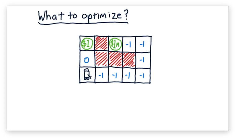
This maze has a reward of $1 two spaces away and a much higher reward of $1 million eight spaces away. The $1 reward is unique in that the robot can receive it multiple times; for instance, entering, exiting, and re-entering the $1 square results in a $2 reward. The robot can only receive the $1 million reward once.

The red squares are obstacles, and the robot cannot occupy those spaces. The other squares are marked with their respective rewards or, in the case of negative numbers, penalties.

Let's say we wanted to optimize the sum of the robot's rewards from now until infinity. We refer to this timeframe as an infinite horizon. In this case, we don't particularly care if the robot exclusively grabs the $1 ad infinitum, or if it first grabs the $1 million before returning to the $1. With regard to the reward, either strategy is sufficient since both result in an infinite reward.

More often than not, we have a finite horizon. We might, for example, want to optimize our reward over the next three moves. If we take three steps towards the $1 million reward, we are going to experience three penalties of -1, for a total penalty of -3. If we take three steps towards the $1, however, we experience a reward of zero, a reward of $1, and a reward of 0, for a total reward of $1.

If we extend our horizon out to eight moves, we see that the optimal path changes. Instead of retrieving the $1 reward four times, we can incur seven penalties of -1 in exchange for the $1 million reward.

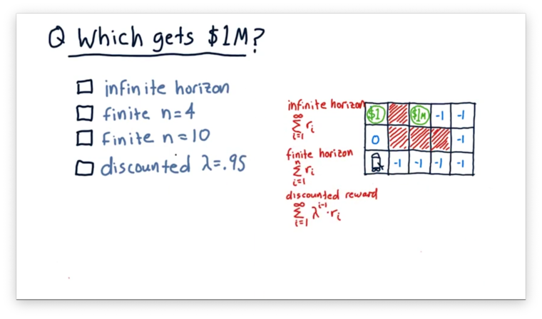
We can now articulate the expression that we want to maximize. Given a horizon of size $n$, and note that $n$ can equal infinity, we want to maximize the expression

Remember from one of our earlier lessons where we talked about the present value and future value of money. One of the main points that we arrived at was that a dollar tomorrow is worth less than a dollar today.

We can think about rewards in a similar fashion: a reward of one dollar today is more valuable than a reward of one dollar tomorrow. We can reformulate our expression above to incorporate the discounting of future rewards. That is, given a discount rate, $\gamma$, we want to maximize

Note: this expression is almost identical to the expression we used to calculate the present value of all future corporate dividend payments.

We can look at the first few terms of this expression to understand what is happening. The value of an immediate reward, $r_1$, is equal to $\gamma^0 * r_1 = r_1$. The value of the next most immediate reward, $r_2$, is equal to $\gamma * r_2$. The value of the third most immediate reward, $r_3$, is equal to $\gamma^2 * r_3$. These first few steps demonstrate how we use $\gamma$ to devalue rewards that are further out in the future.

The value of $\gamma$ is greater than zero and less than or equal to one. The closer it is to one, the more we value rewards in the future (the less we discount them). The closer it is to zero, the less we value rewards in the future (the more we discount them).

Which Approach Gets $1M Quiz

Which of the following approaches leads our robot to a policy that causes it to reach the $1 million reward?

Which Approach Gets $1M Quiz Solution

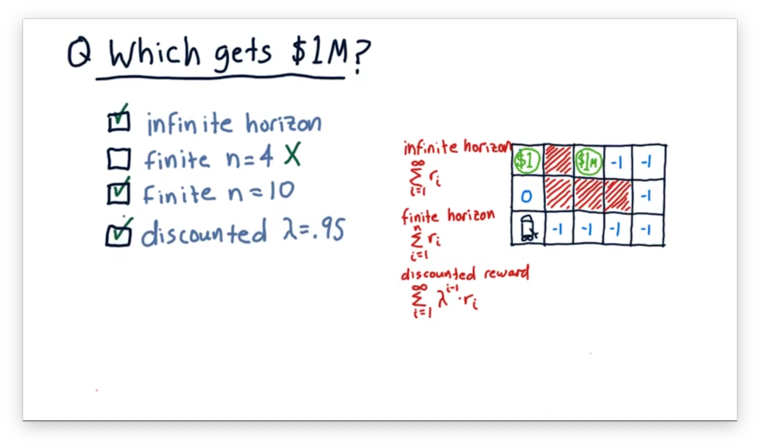
With an infinite horizon, the robot may exclusively grab the $1 ad infinitum, or it might first grab the $1 million before returning to the $1. As a result, obtaining the $1 million is possible with infinite horizon, but not guaranteed.

With a finite horizon of length four, the robot does not reach the $1 million. A journey towards the $1 million results in four penalties, whereas heading towards the $1 results in a positive reward. However, if we increase the horizon to ten, the robot does reach the $1 million.

In the discounted scenario, each reward in the future is successively devalued by 5%. Even so, the $1 million reward is so large that seeking this reward is still the optimal strategy.